18 IS-MP – ECO 1000 Lecture Notes

Objectives

Understand relationship between the interest rate and different components of aggregate expenditure (IS Curve)
Identify movements along vs. shifts of the IS curve
Understand MP curve and its components
1. Risk-free rate
2. Risk premium
Identify macro equilibrium

18.1 Introduction

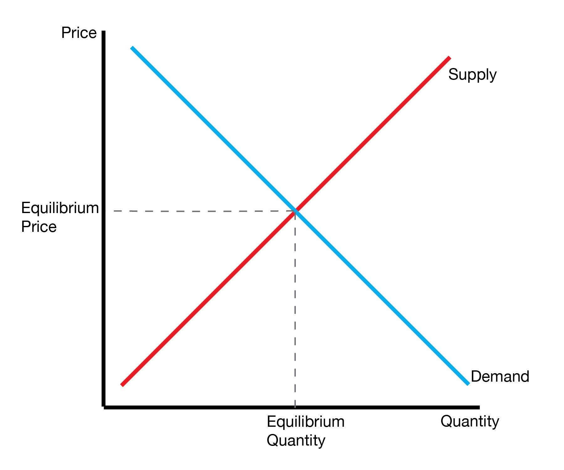
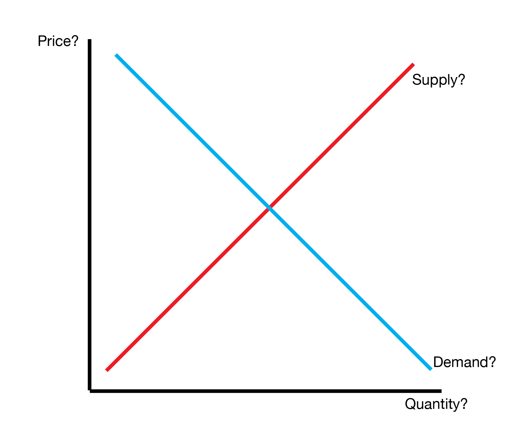
This lecture introduces our concept of a macro equilibrium, a quantity and price for the overall macro economy. Until now, we’ve focused on microeconomics equilibria, the quantity and prices for individual goods such as bread and computers. The main leap is deciding on our price and quantity.

18.2 Macro Demand: IS Curve

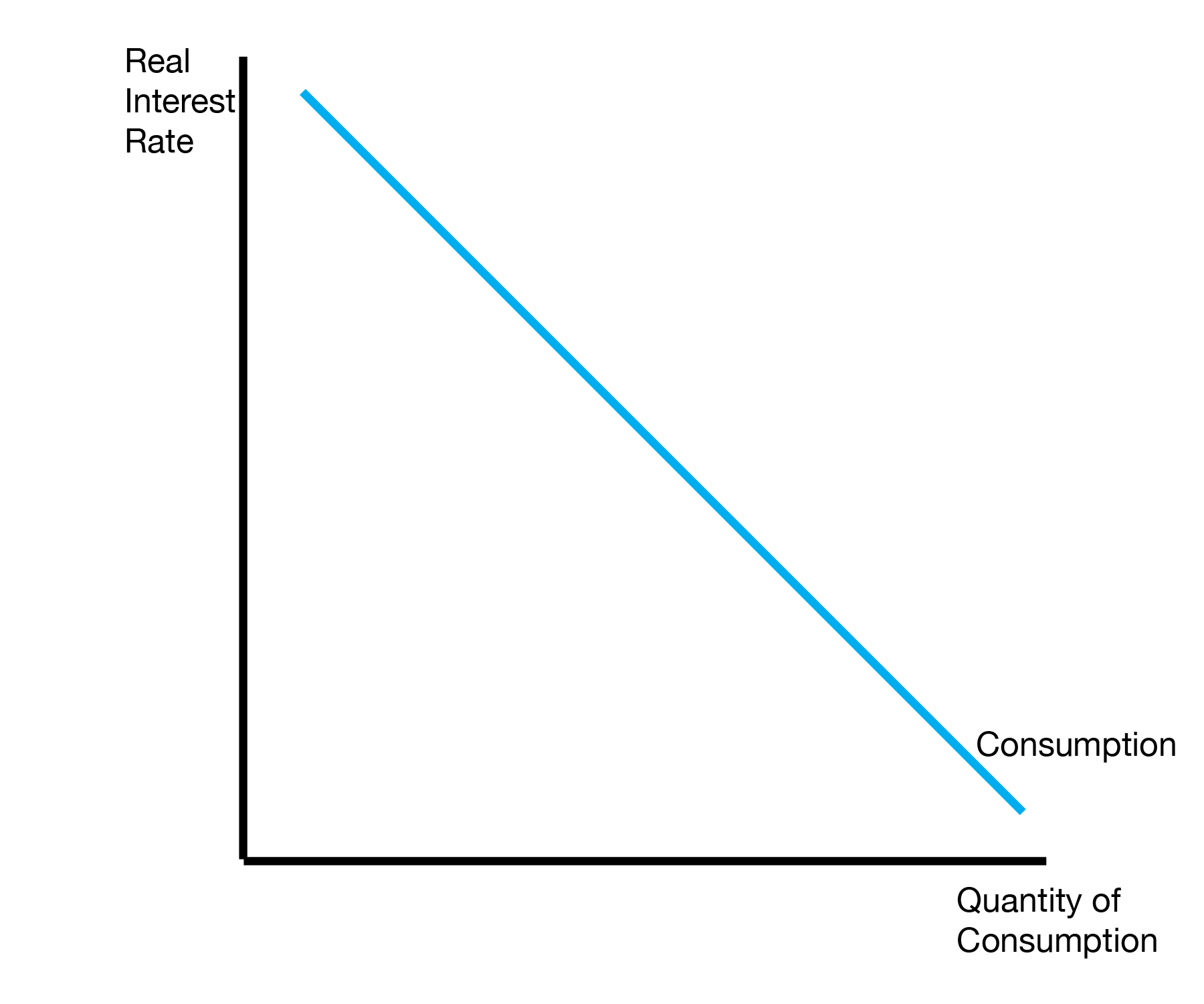
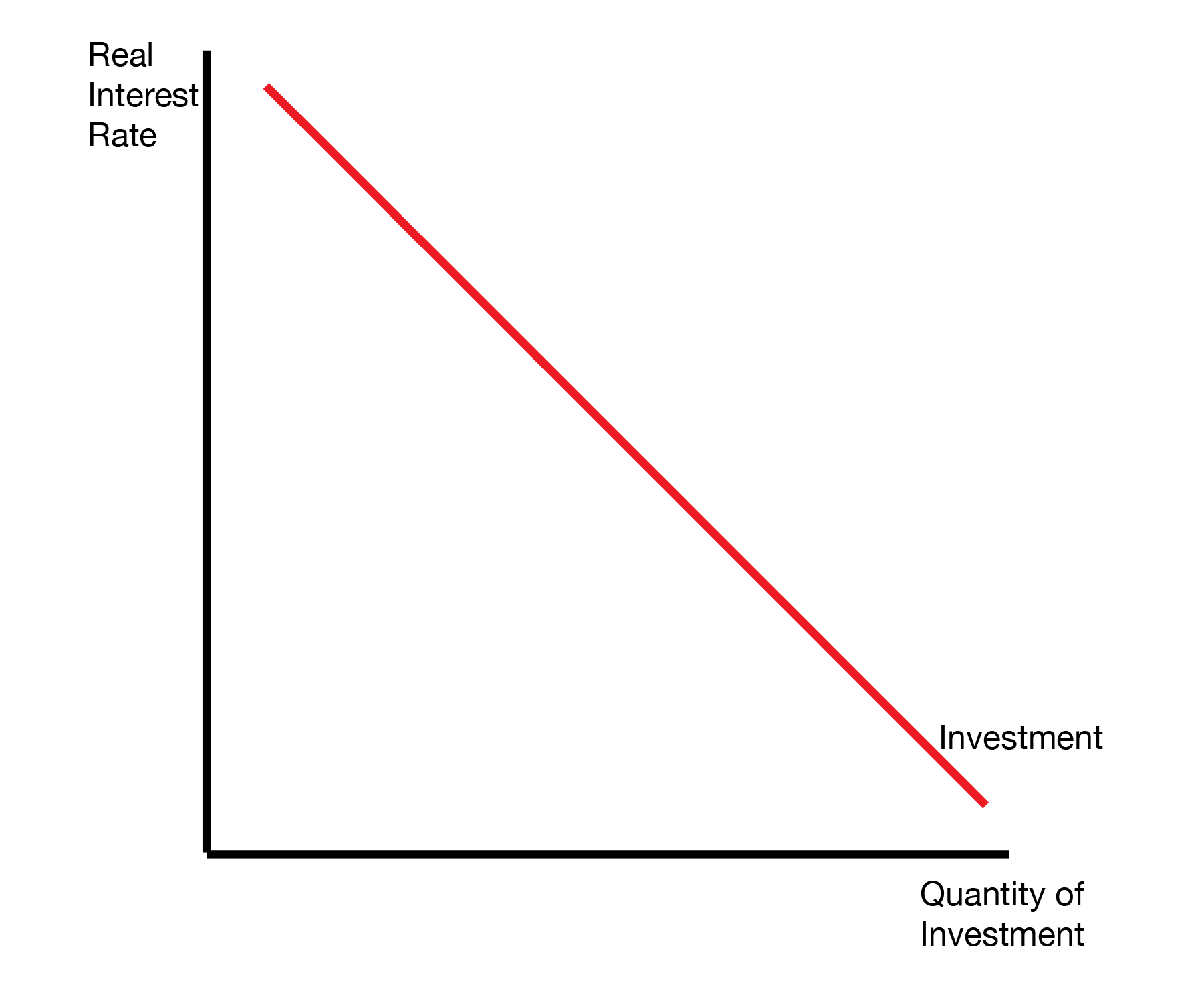
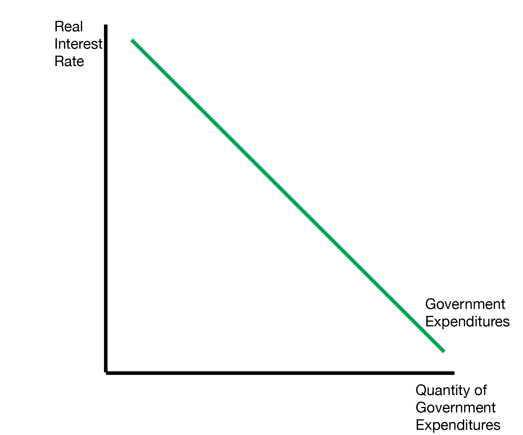
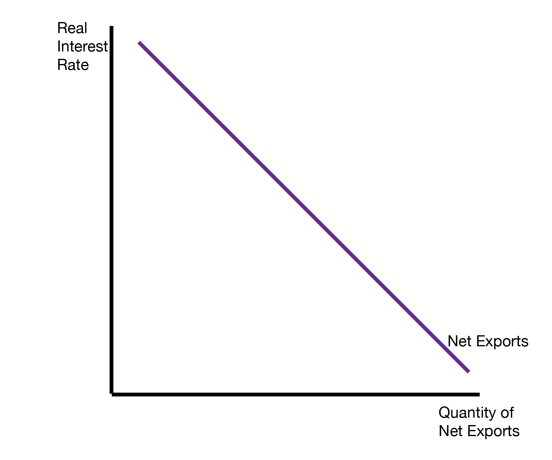
This section examines the relationship between the interest rate and the four components of GDP. Each component features a decreasing relationship with the interest rate. For consumption, this occurs because households want to save more when the interest rate is higher. For investment, this occurs because it is more expensive to finance new projects when the interest rate is higher. For government expenditures, it is more expensive for the government to spend (and borrow) when the interest rate is higher.

Interest Rate and Government Expenditures

18.2.1 Aggregate Expenditure and Output Gap

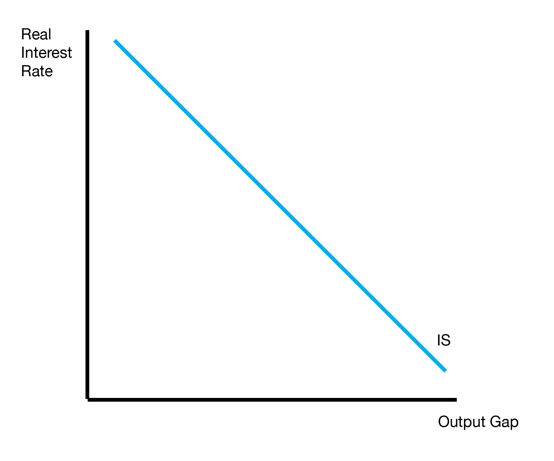
Conveniently, all components of GDP have a decreasing relationship with the interest rate. When added together, GDP as a whole has a decreasing relationship with the interest rate. Finally, if we compute the output gap, the output gap has a decreasing relationship because it is proportional to actual GDP.

When expressed graphically, this gives the IS curve:

IS Curve

For each interest rate, the resulting output gap.

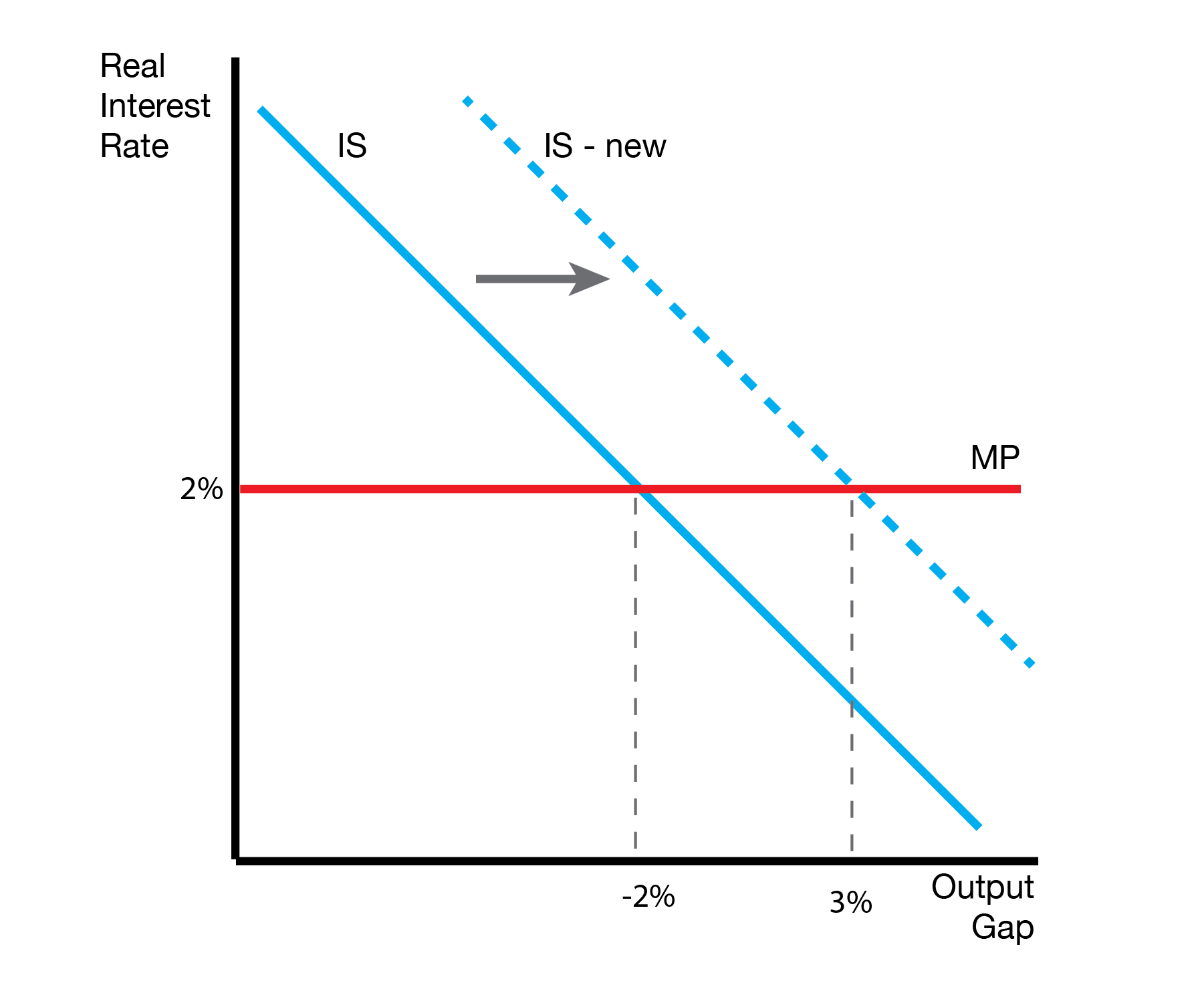
18.2.2 Shifts

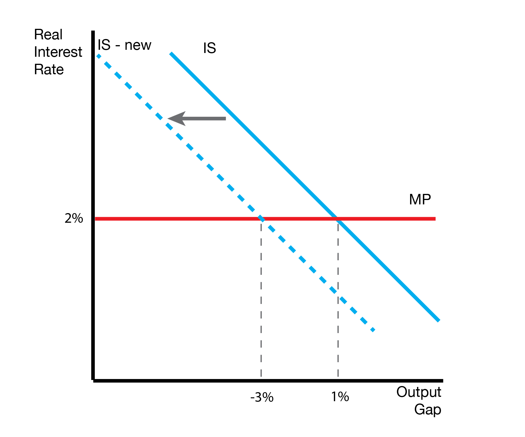
Once we’ve developed our IS curve, we can develop shifts in the IS curve. No different than microeconomics, if anything other than the price changes, the curve shifts. In this case, the price is the real interest rate, so if anything other than the real interest rate changes, it produces a shift in the IS curve.

18.3 Macro Supply: MP Curve

We developed the IS curve, our notion of ‘demand’ in the macro economy. We will now develop our notion of supply.

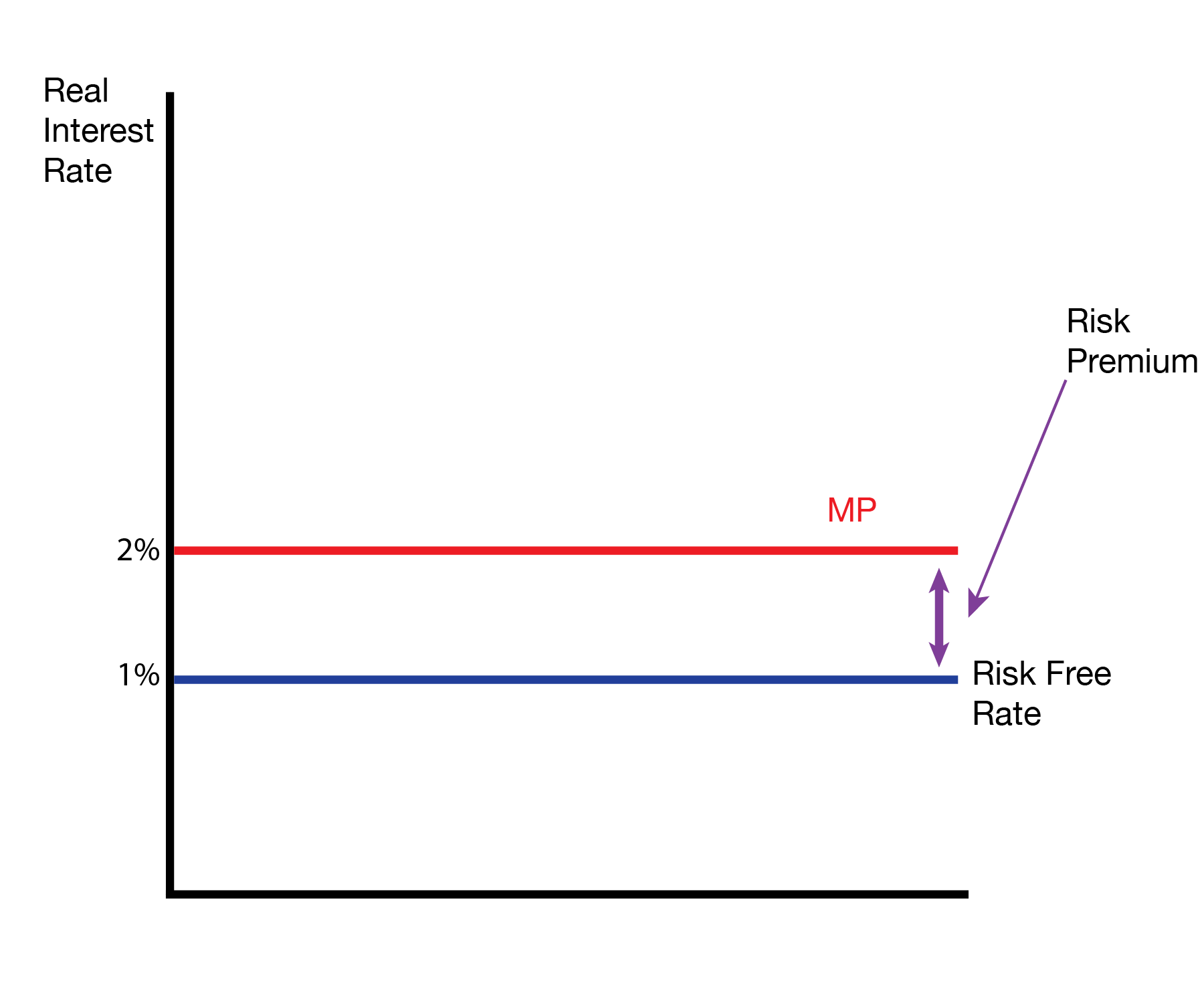
The MP curve captures the interest rate of the economy. It features two components: the risk free rate of interest, which is set by the central bank, and the risk premium, which is added by the financial industry. Graphically, the MP curve is horizontal: the interest rate is independent of the output gap.

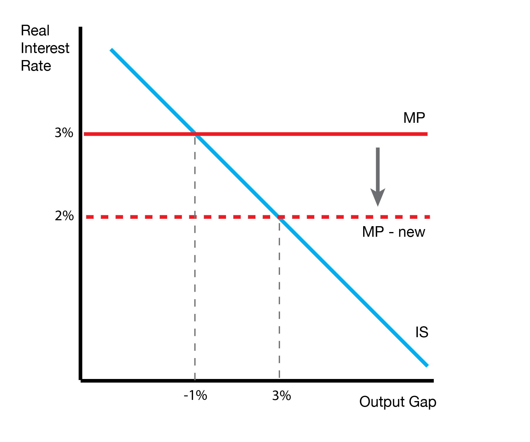
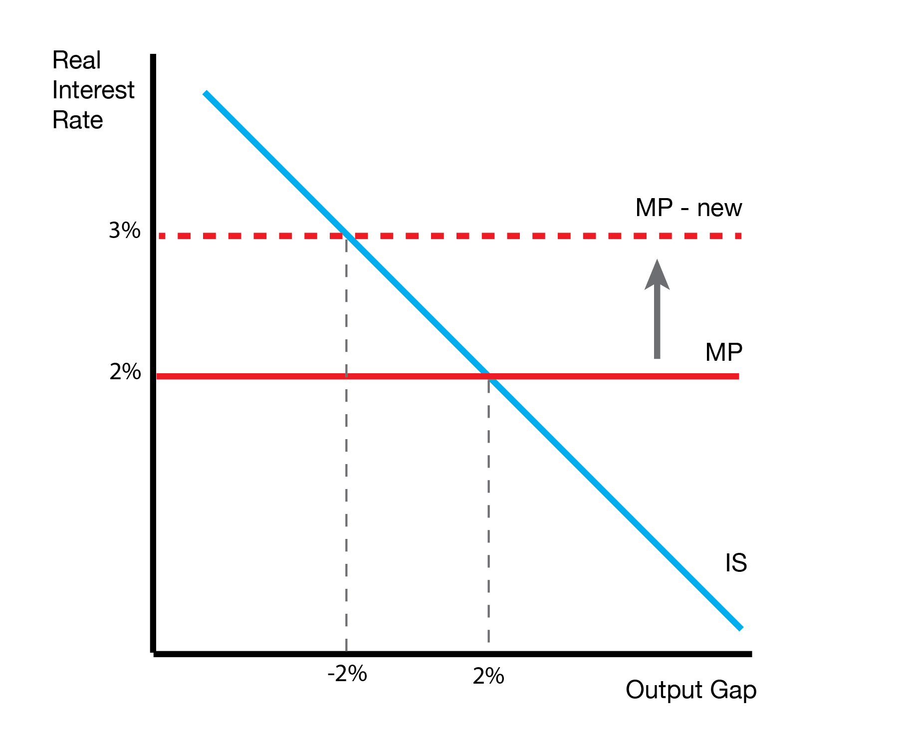
18.3.1 Shifts

Now that we developed the MP curve, we can introduce ‘shifts’ to the MP curve. Graphically, these can be seen as vertical increases or decreases in the MP curve (real interest rate).

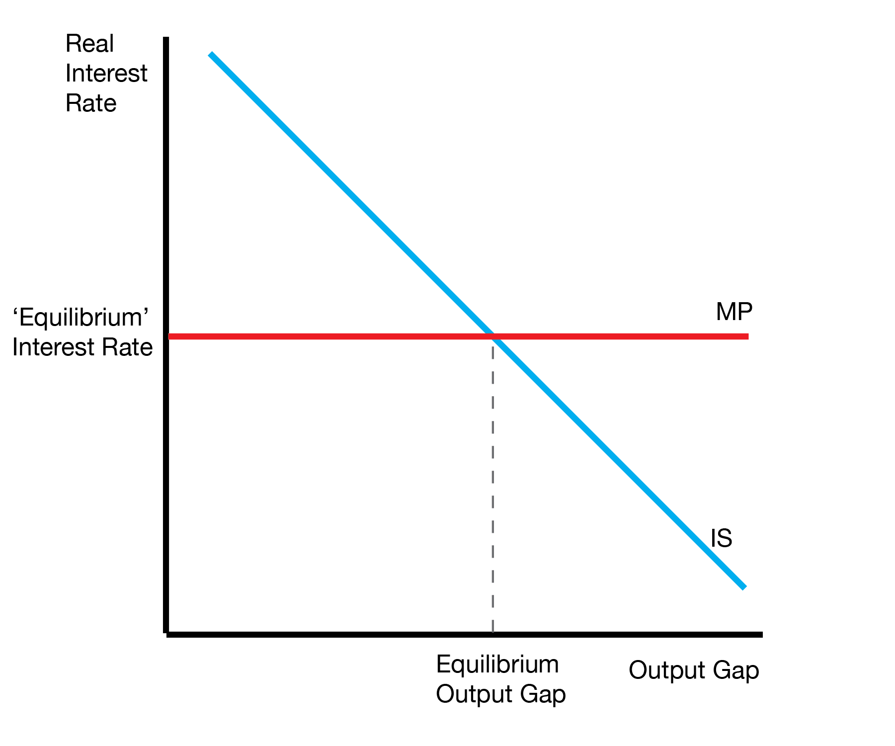
18.4 Equilibrium

Now that we’ve developed our macro demand (IS curve) and macro supply (MP curve), we can develop our macro equilibrium. The IS-MP equilibrium simply combines the IS and MP curves. The equilibrium price is the real interest rate. The equilibrium quantity is the output gap.

We can view the equilibrium interest rate as being ‘forced’ by the central bank’s choice of MP curve. Given the MP curve, the equilibrium output gap is given by the interesection of the IS and MP curve.

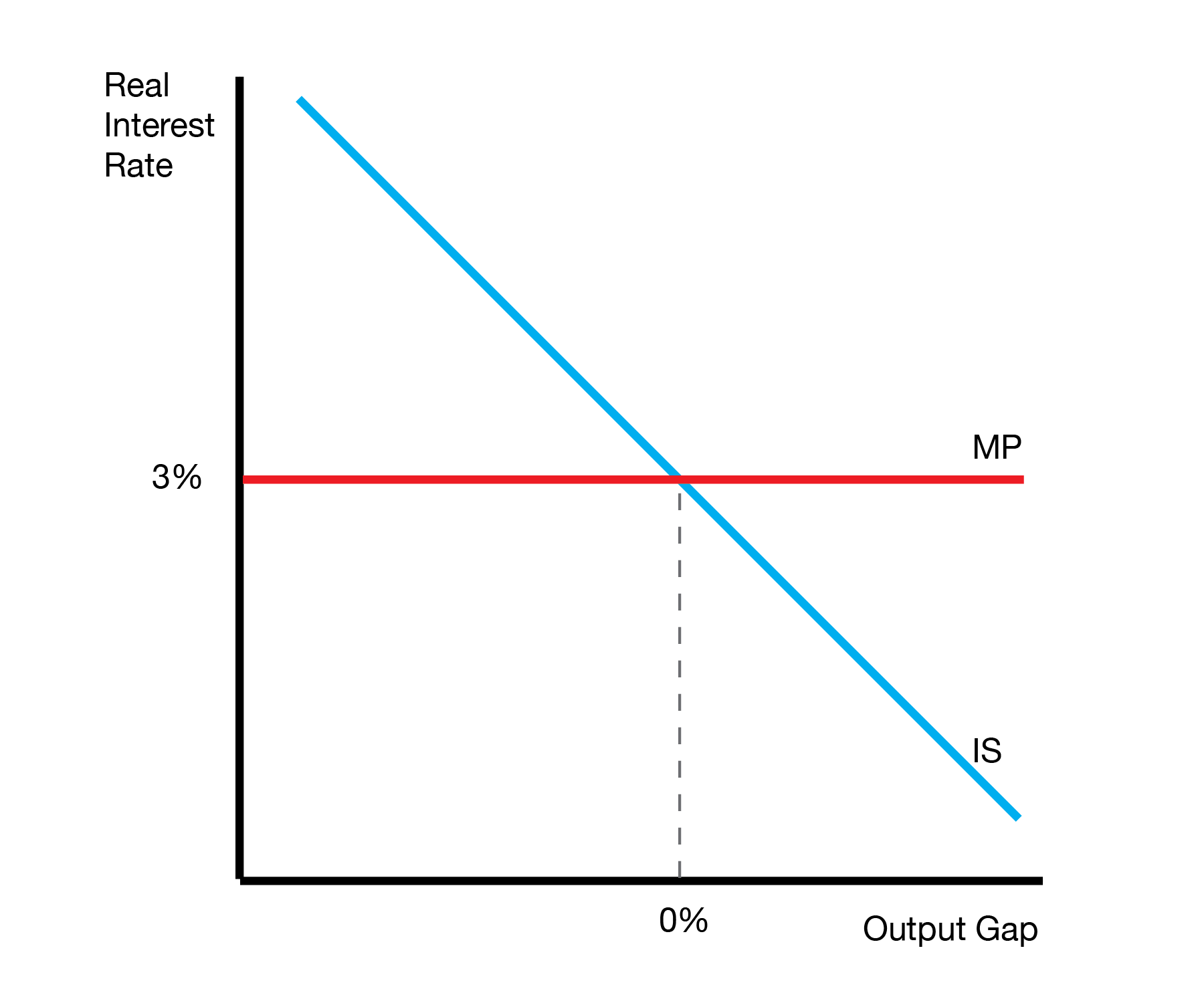
For example, when the central bank sets the MP curve to 3%, we can examine the IS curve to see the resulting output gap is 0%.

18.5 Conclusion

This lecture introduces the IS-MP model, our model of macroeconomic equilibrium
The overall demand of the economy is given by the IS curve
With the addition of the MP curve, we have a unique equilibrium interest rate and output gap