9 IS-LM-FX Model
Objectives
- Solve goods market equilibrium and produce resulting IS curve
- Identify IS curve shifts
- Solve money market equilibrium and produce resulting LM curve
- Identify LM curve shifts
- Understand order of operations for floating and fixed exchange rate regimes
- Identify optimal fiscal response to booms and busts
- Identify optimal monetary response to booms and busts
- Understand the tradeoffs presented by the zero lower bound
This section develops the IS-LM-FX model. This model is an extension of the MM-FX model which endogenizes output \(Y\). That is, output \(Y\) will be an endogenous result of the model rather than an exogenous shock.
9.1 Goods Market
Now that \(Y\) is a ‘free’ variable in the model, we need to know where it comes from. More specifically, we have to give the model more structure so that we actually know the value of \(Y\). We will do this using the Goods Market.
The Goods Market captures the demand for all goods in the economy. It features the demand from consumption, investment, the government, and net exports.
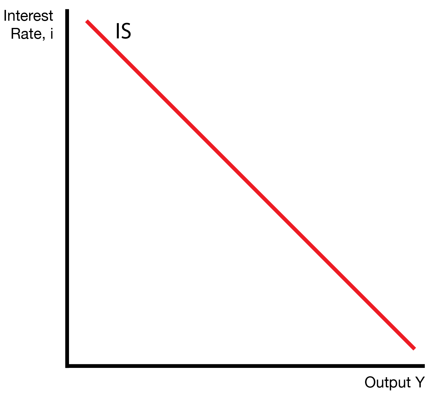
9.2 IS Curve
This section presents the IS curve. We need equilibrium in three markets: the foreign exchange market, goods market, and money market. The IS curve will bring equilibrium to the foreign exchange and goods markets.
9.2.1 Derivation
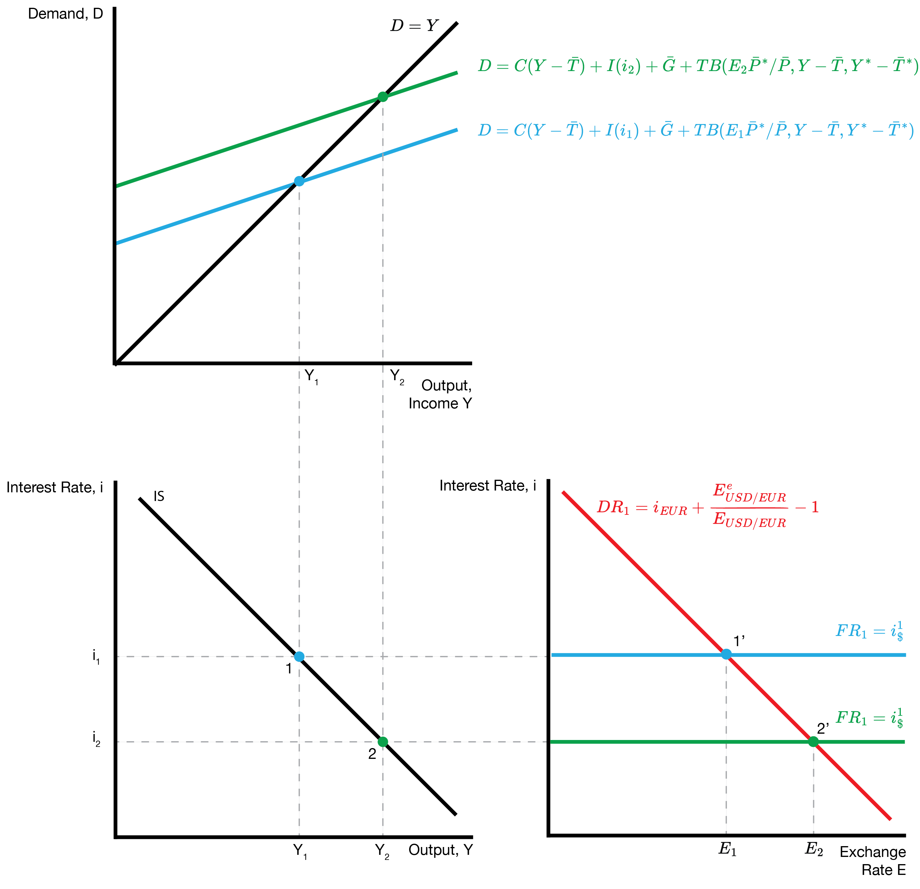
For a single interest rate \(i_1\), we solve for the output \(Y_1\) that results if both the goods and foreign exchange market are in equilibrium. Notice that the goods market itself depends on the exchange rate \(E\). Because of this, we will visit the foreign exchange market first so that we know the exchange rate \(E_1\) ahead of time.
We then visit the goods market. Given our interest rate \(i_1\) and exchange rate \(E_1\), we find the unique output \(Y_1\) that is consistent with the goods market clearing. This provides a single point for our IS curve.
We derive the rest of the IS curve by solving for a new point given a lower interest rate \(i_2\). Revisiting the foreign exchange and goods markets provides a higher output \(Y_2\), which shows that the IS curve is decreasing.
9.2.2 Shifts
We now examine shifts of the IS curve. A ‘shift’ occurs when anything other than the interest rate changes.
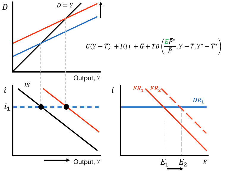
In this example, we consider an increase in the expected future exchange rate \(E^e\). We first visit the foreign exchange market to see how the increase in \(E^e\) changes the equilibrium exchange rate \(E\). We then visit the goods market to see how the increase in \(E^e\) changes the equilibrium output \(Y\). The increase in demand for exports (from foreign) increases the overall demand for goods, which increases output \(Y\).
We’ve shown this is true for \(i_1\), but the same logic applies for any interest rate. As a result, the entire IS curve shifts to the right (increases) for an increase in \(E^e\).
The following table summarizes how shifters can drive an increase (rightward shift) of the IS curve.
| IS Shifters (Increase) |
|---|
| Fall in taxes \(\bar{T}\) |
| Rise in government spending \(\bar{G}\) |
| Rise in foreign interest rate \(i^*\) |
| Rise in future expected exchange rate \(E^e\) |
| Rise in foreign prices \(P^*\) |
| Fall in home prices \(P\) |
| Any shift up in the consumption function \(C\) |
| Any shift up in the investment function \(I\) |
| Any shift up in the trade balance function \(TB\) |
9.3 LM Curve
This section develops the LM curve. The IS curve ensures equilibrium in the goods and foreign exchange markets, but we still need to ensure equilibrium in the money market. The LM curve captures equilibrium in the money market.
Once we allow for its intersection with the IS curve, we will have equilibrium in all three markets: goods, foreign exchange, and money.
9.3.1 Derivation
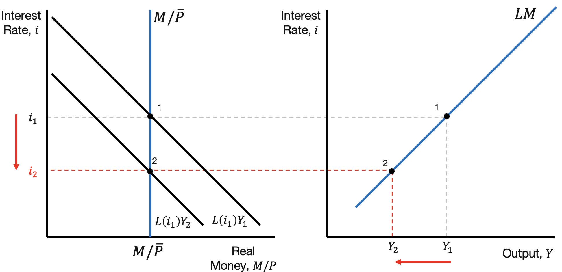
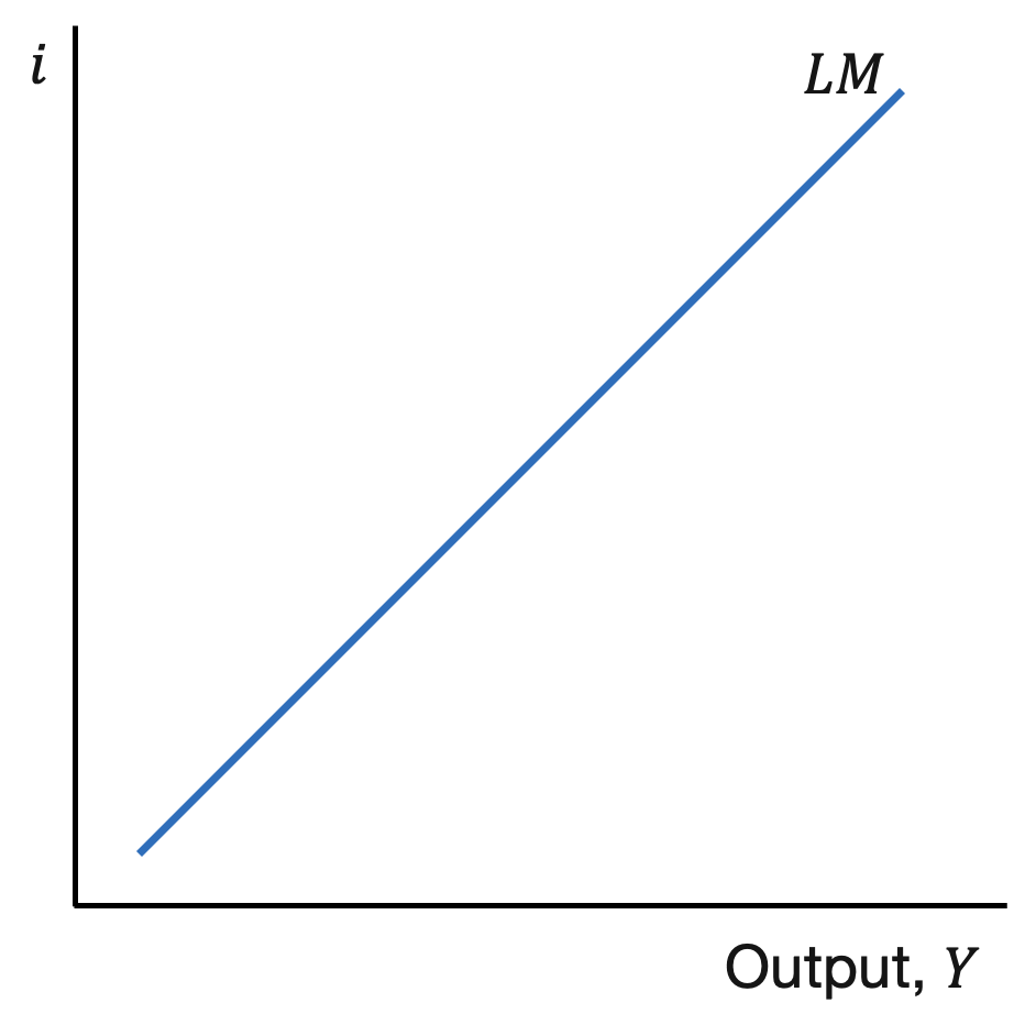
We first fix the interest rate \(i_1\) and find the unique output \(Y_1\) that clears the money market. Real money demand \(L(i_1) Y\) is increasing in \(Y\). This provides our unique output \(Y_1\).
We solve for the rest of the LM curve by examining how \(Y\) changes for a decrease in the interest rate. This reveals that the LM curve is increasing in the interest rate \(i\).
9.3.2 Shifts
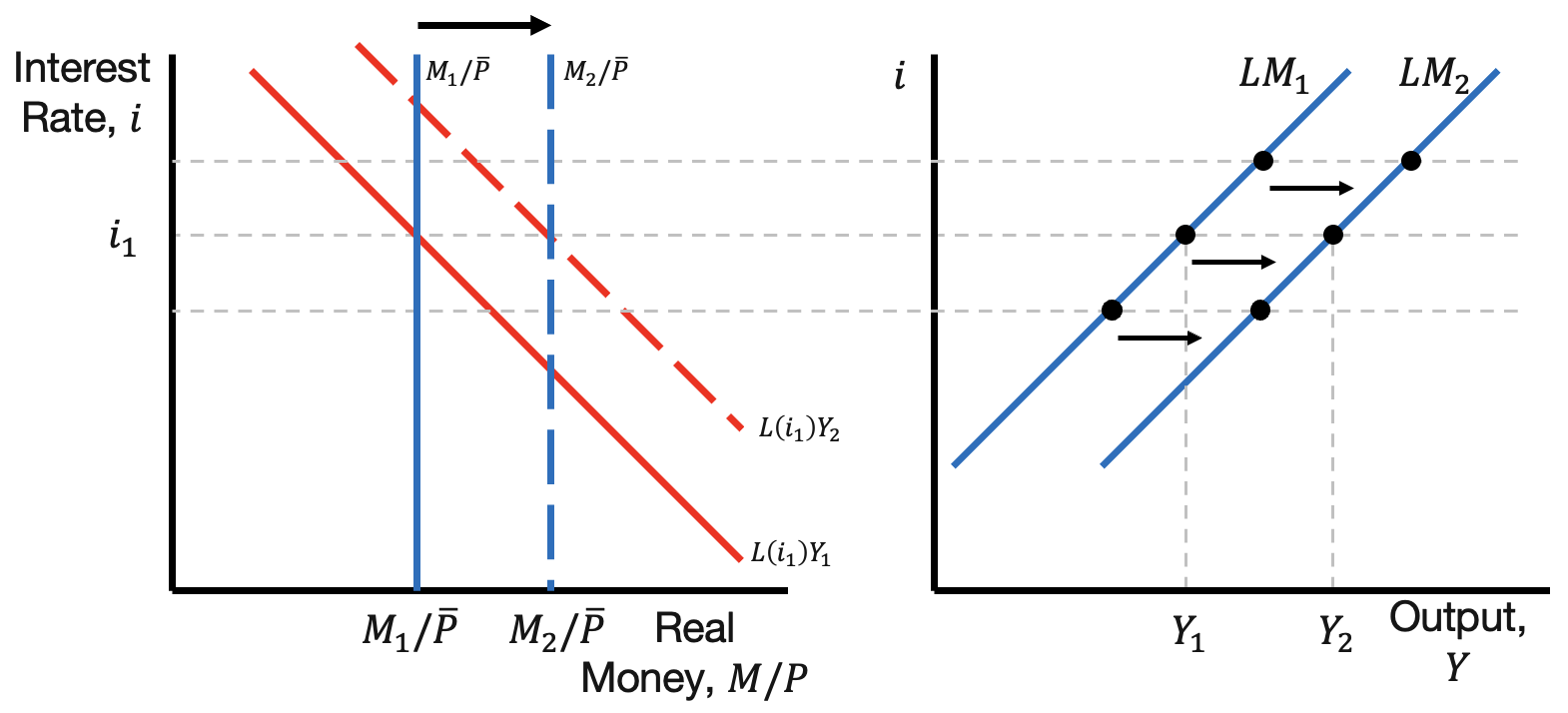
We now examine shifts of the LM curve. Our methodology is as follows. For a given interest rate \(i_1\), there is a unique output \(Y_1\) that is consistent with the money market clearing.
Our next step is to introduce the shifter (change in money supply \(M\) or demand function \(L\)), and examine how \(Y_1\) changes for \(i_1\). Finally, because interest rate \(i_1\) is not ‘special’, the same shift happens for every interest rate: e.g. the entire curve shifts.
| LM Shifters (Increase) |
|---|
| Rise in (nominal) money supply \(M\) |
| Any shift left in the money demand function \(L\) |
The primary shifters are the money supply \(M\) and the money demand function \(L\).
9.4 Equilibrium
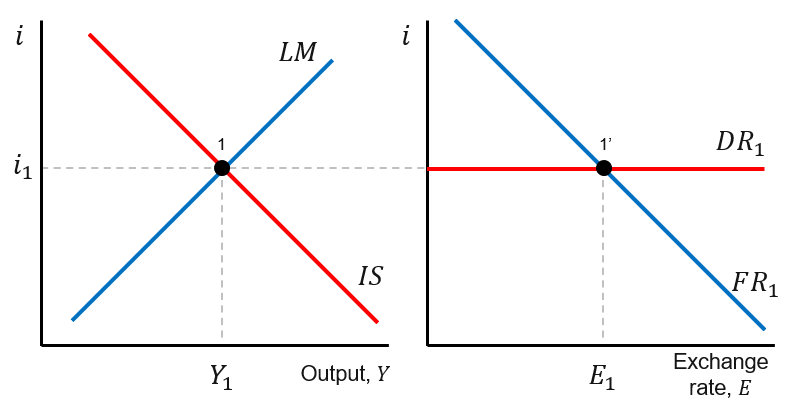
We now combine the IS and LM curves to form our equilibrium. Their intersection represents the interest rate \(i\) and output \(Y\) that is consistent with the goods, money, and foreign exchange (FX) markets clearing.
This provides our equilibrium interest rate \(i_1\), output \(Y_1\), and exchange rate \(E_1\).
9.5 Policy
This section examines policy in the IS-LM-FX model. The model features two forms of policy: fiscal policy, which controls government spending \(G\) and taxes \(T\), and monetary policy, which controls money supply \(M\).
| Policy Type | Tool | Effect on IS/LM |
|---|---|---|
| Fiscal | Government spending \(G\), Taxes \(T\) | Shifts IS curve |
| Monetary | Money supply \(M\) | Shifts LM curve |
Notice that government spending \(G\) and taxes \(T\) are fiscal policy tools because they directly influence the goods market. Moreover, they have no influence on the money market, so they only shift the IS curve. On the other hand, the money supply \(M\) influences the money market. It has no influence on the goods market, so it only shifts the LM curve.
9.5.1 Fiscal
This section examines a fiscal expansion under floating and fixed exchange rate regimes.
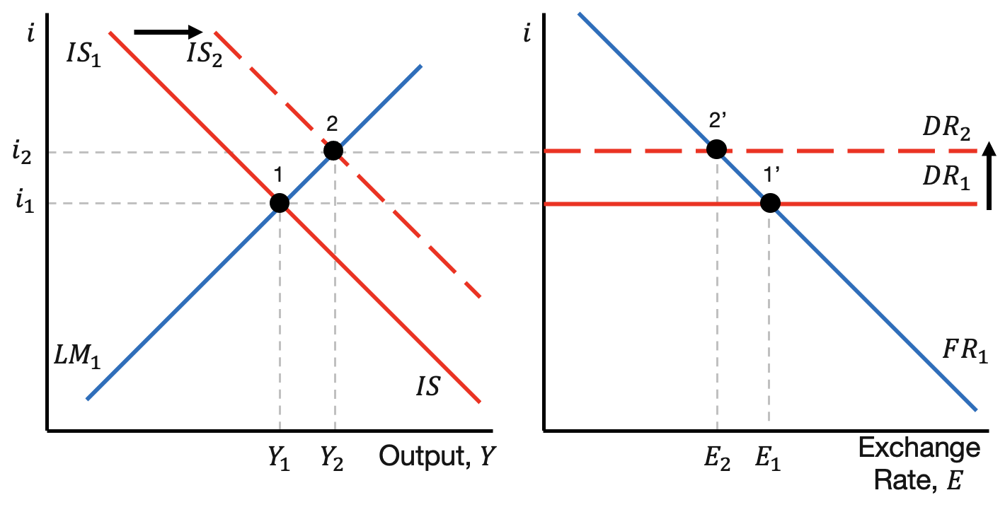
We first examine a fiscal expansion under a floating exchange rate. The increase in government spending \(G\) leads to a rightward shift (increase) of the IS curve. This drives an increase in the interest rate and increase in output. Next, we carry the higher interest rate to the FX market, which produces an increase in the domestic return \(DR\) curve. This leads to a decrease (appreciation) of the exchange rate \(E\).
We now examine a fiscal expansion under a fixed exchange rate regime. As before, the increase in spending drives an increase in the interest rate and output. The higher interest rate drives an exchange rate appreciation.
The fixed exchange rate differs in that it will respond to the exchange rate appreciation. That is, the central bank needs to get the exchange rate back to its target value \(\bar{E}\). Equivalently, the central bank needs to return the interest rate to its original lower value. Its tool to do this is the LM curve, which is influenced by the money supply. The central bank prints money to increase the LM curve. This lowers the interest rate, which restores the equilibrium exchange rate to its original value.
Under the fixed exchange rate, expansionary fiscal policy leads to a larger increase in output \(Y\). This occurs because the initial increase in government spending changes the exchange rate, which forces the central bank’s hand.
9.5.2 Monetary
This section examines a monetary expansion under floating and fixed exchange rate regimes.
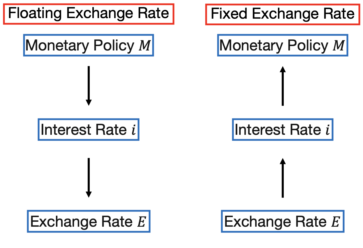 The primary focus is whether the economy is following a floating or fixed exchange rate regime. Under a floating exchange rate regime, the monetary authority sets the money supply. Within the IS-LM market, this determines the home interest rate. Within the FX market, the home interest rate determines the equilibrium exchange rate.
Under a fixed exchange rate regime, we follow the reverse path. The monetary authority has an exchange rate target \(\bar{E}\). Examining the foreign exchange market, this forces them to have a certain interest rate \(i\). The monetary authority then has to manipulate the money supply \(M\) so that \(i\) is the resulting equilibrium interest rate.
We first examine monetary expansion under a floating exchange rate regime. The increase in money supply leads to a rightward shift of the LM curve. This results in a lower equilibrium interest rate and higher level of output. We now carry the lower interest rate to the FX market. The lower interest rate produces an exchange rate depreciation (Home currency has a lower return, so Home currency is less valuable).
Next, we examine monetary expansion under a fixed exchange rate. The central bank increases the money supply \(M\), producing a rightward shift of the LM curve and decrease in the interest rate. The decrease in the interest rate leads to a depreciation of the exchange rate, breaking the fixed exchange rate. This forces the central bank to reverse course. The central bank then cuts back on the money supply to recover the interest rate and exchange rate. This provides an important lesson: under a fixed exchange rate, monetary policy is ineffective because the central bank is preoccupied with maintaining the exchange rate target \(\bar{E}\).
9.6 Optimal Policy
This section studies optimal fiscal and monetary policy.
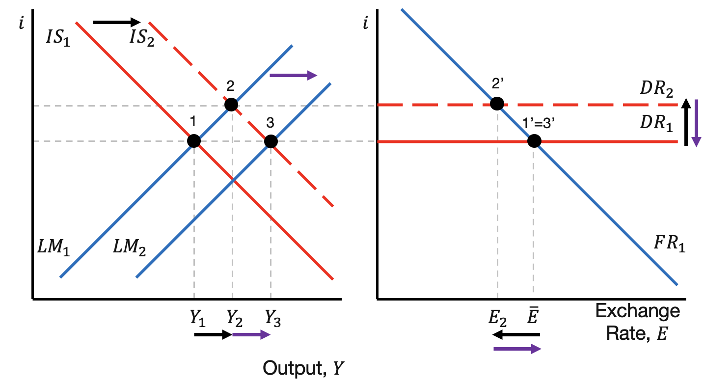
9.6.1 Bust
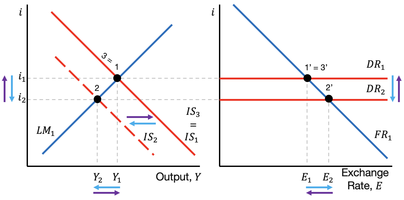
We first examine fiscal policy during a bust episode. The bust episode is represented by the leftward shift (contraction) of the IS curve to \(IS_2\). This puts the domestic market at equilibrium point 2 and the FX market at equilibrium point 2’. The government increases spending. Through the goods market, this shifts the IS curve rightward to the original equilibrium point 1. Similarly, the FX market returns to its original equilibrium point 3’ = 1’.
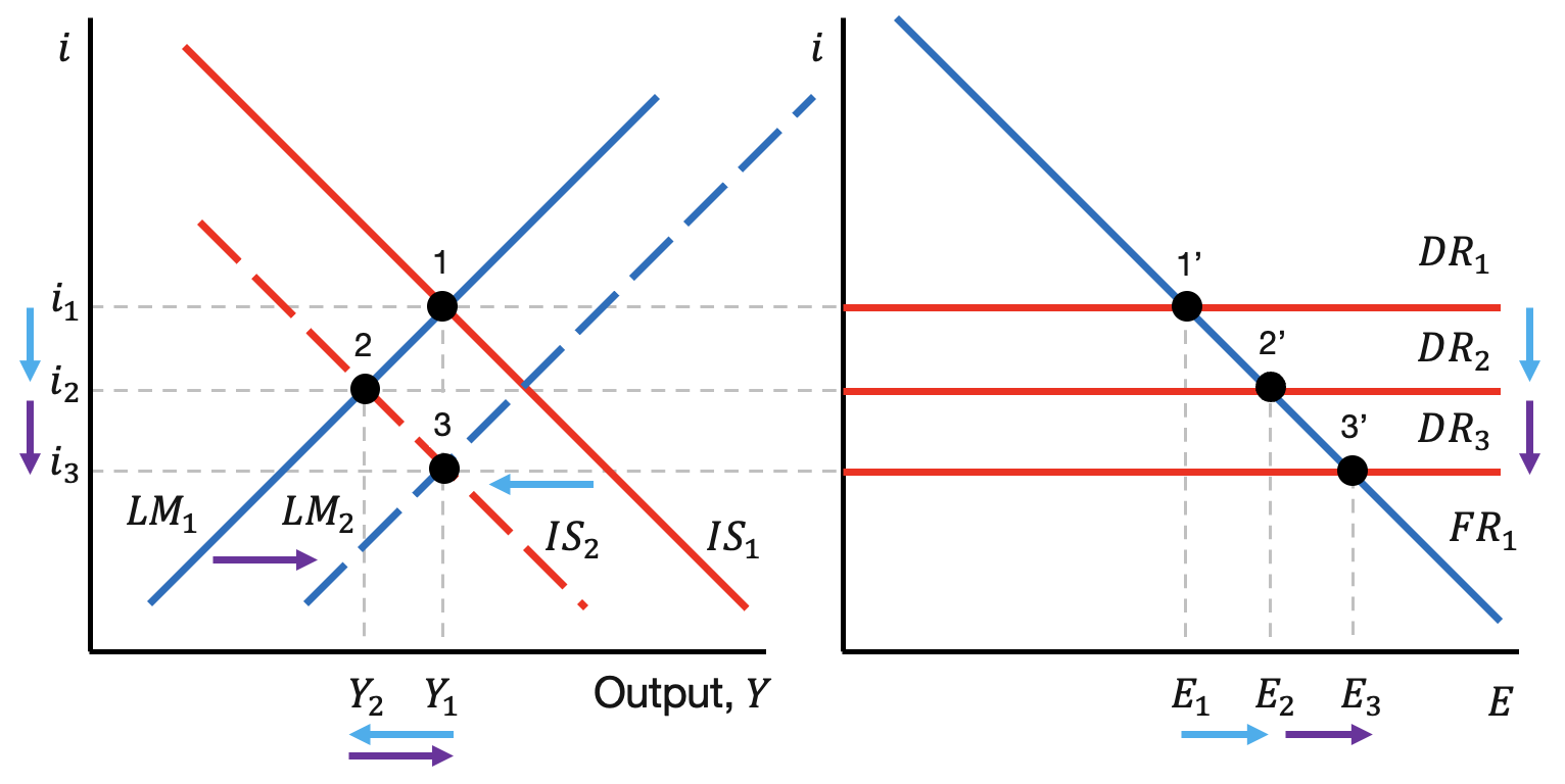
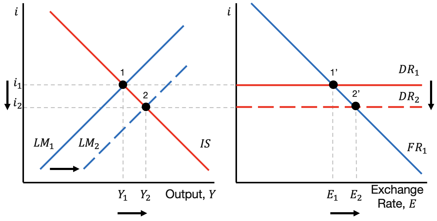
Next, we examine monetary policy during a bust episode with a floating exchange rate. The bust leads to a leftward shift of the IS curve, putting the economy at equilibria 2 and 2’, respectively. The monetary authority (central bank) increases the money supply to drive a rightward shift (increase) of the \(LM\) curve to \(LM_2\). This puts the economy at equilibrium point 3, which features a lower interest rate but brings the economy back to its original output level \(Y_1\).
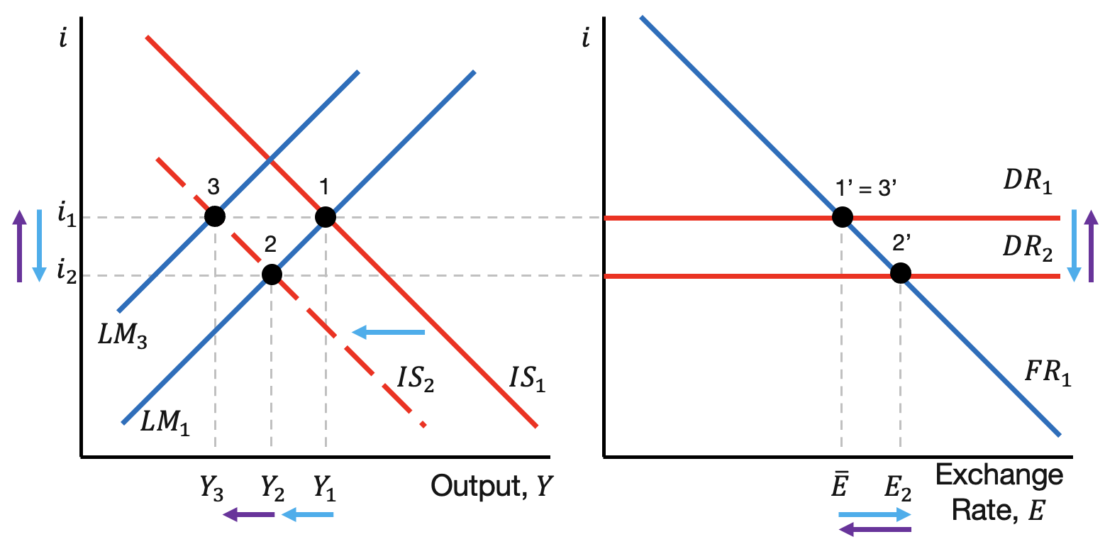
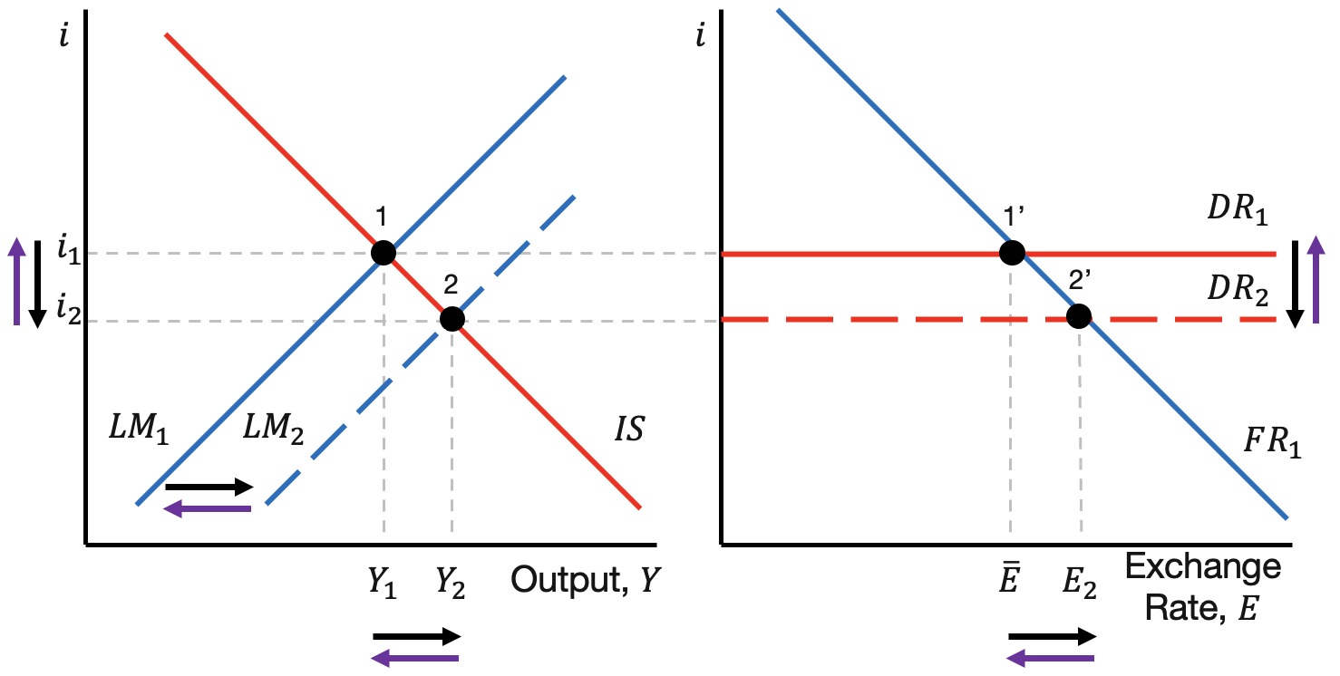
Lastly, we examine monetary policy during a bust episode with a fixed exchange rate. The initial bust in the economy (\(IS\) moving to \(IS_2\)) leads to a depreciation in the exchange rate market. To return to the exchange rate target \(\bar{E}\) , the monetary authority needs to increase the interest rate to its original level \(i_1\). To do this, they contract the money supply, which produces a decrease in the \(LM\) curve and increase in the interest rate. This restores the exchange rate to its target \(\bar{E}\). Within the domestic market, this further decreases output to a lower level. Therefore, the monetary authority brings stability to the exchange rate market, but amplifies the downturn in the domestic market.
9.7 Conclusion
- This lecture develops the goods market to endogenize output.
- We combine the Goods and FX markets into the IS curve.
- We study the responses to different shocks within the IS-LM and FX markets.
- We study the optimal responses of fiscal and monetary policy under floating and fixed exchange rates.