3 Heckscher-Ohlin Model
Objectives
- Build trade equilibrium in the Heckscher-Ohlin model
- Understand the Stolper-Samuelson theorem
- Be able to identify winners and losers based on factor abundance
3.1 Introduction
This lecture introduces the Heckscher-Ohlin model of trade. The Heckscher-Ohlin model builds on the Ricardian model by introducing another factor of production, capital. This improves the Ricardian model, which is unable to have a ‘loser’ from trade because it features one factor of production( labor). In addition, the Heckscher-Ohlin model features a different driver of trade. Trade in the Ricardian model is driven by differences in productivity. We will see that trade in the Heckscher-Ohlin model is driven by different amounts of factors.
3.2 Structure
We will assume Home has a stock of labor \(\overline{L}\) and a stock of capital \(\overline{K}\). Each factor of production is used in two industries: computers (C) and shoes (S). We will assume both goods are produced using both factors of production, and the factors can move freely across industries.
Because we allow for free movement across industries, we view the Heckscher-Ohlin model as capturing the long run rather than the short run. The idea is that in the short run, capital and labor can’t refactor into different industries: machines are built for a specific industry and workers are trained for a specific industry. In the long run, we build new machines and train new workers, so they can move freely across industries.
We represent this as the following equations: \[ \begin{aligned} \overline{L} &= L_C + L_S \\ \overline{K} &= K_C + K_S. \end{aligned} \] The total stock of labor is used in the computer industry (\(L_C\)) and the shoe industry (\(L_S\)), and similarly for capital.
We will assume shoes are labor intensive and computers are capital intensive. The labor intensity of shoes is given by the assumption \[ \frac{L_S}{K_S} > \frac{L_C}{K_C}, \]
that is shoes use relatively more labor than computers. Note this only refers to the relative ‘recepie’ to make one pair of shoes or one computer. We aren’t pinning down the ‘total’ amount of capital or labor needed.
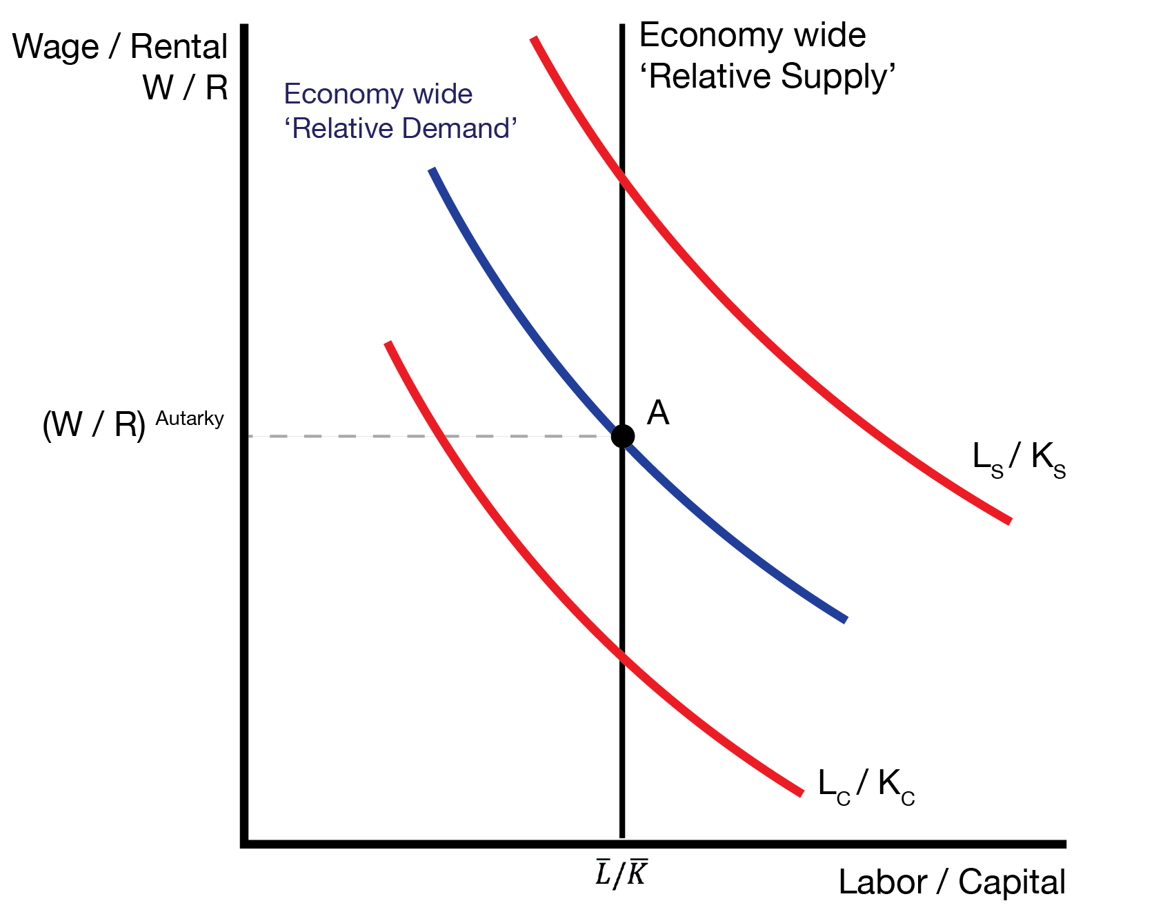
We express this graphically using the relative demand graph:
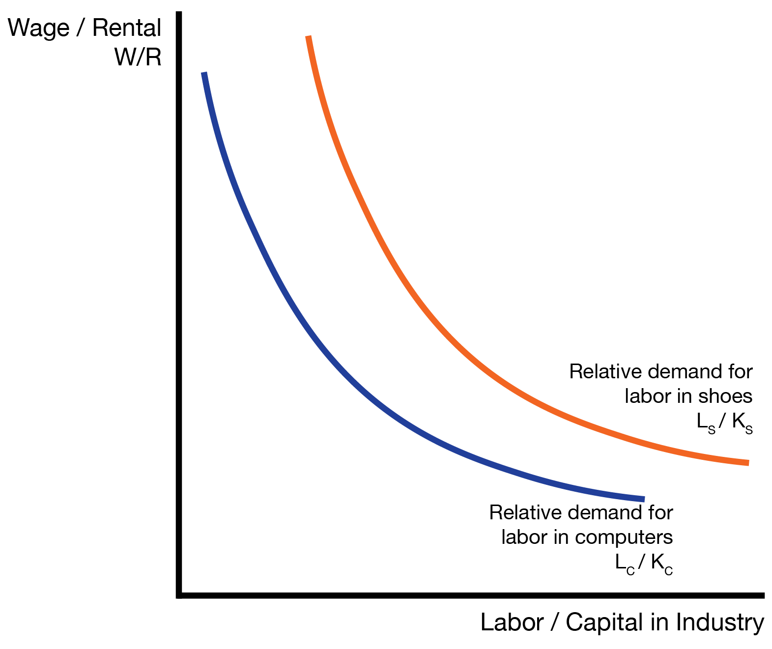
For a given ‘relative price of labor’ \(W/R\), the shoe industry demand ‘relatively’ more labor than the computer industry, \(L_S/K_S > L_C/K_C\).
We also need to consider foreign, who has their own labor and capital stocks \(\overline{L}^*\) and \(\overline{K}^*\).
We will assume Home is capital abundant and Foreign is labor abundant: \[ \frac{\overline{K}}{\overline{L}} > \frac{\overline{K}^*}{\overline{L}^*}. \]
This means home has ‘relatively’ more capital than foreign. Focusing on the ‘relative’ sizes of labor and capital is critical because it allows us to compare different sizes of countries, say Switzerland and Portugal compared to China and India.
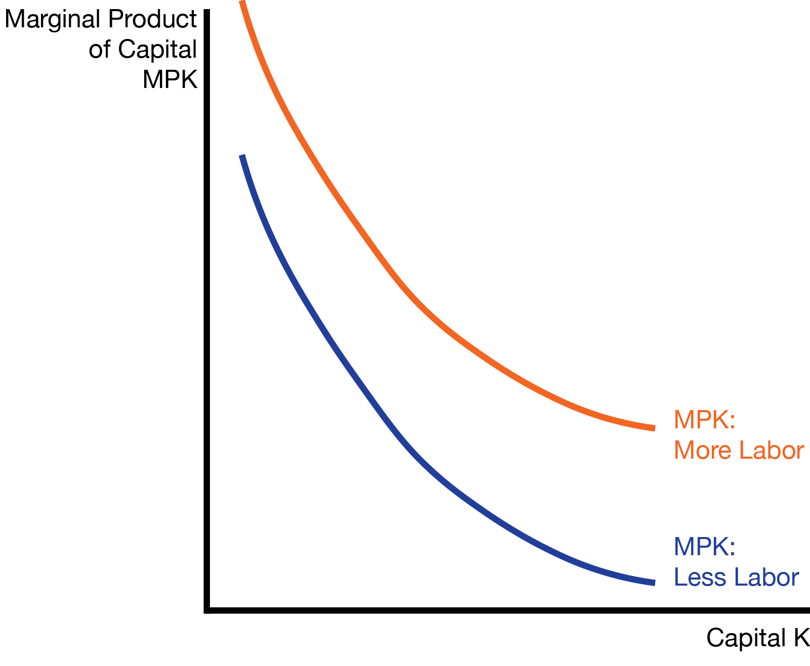
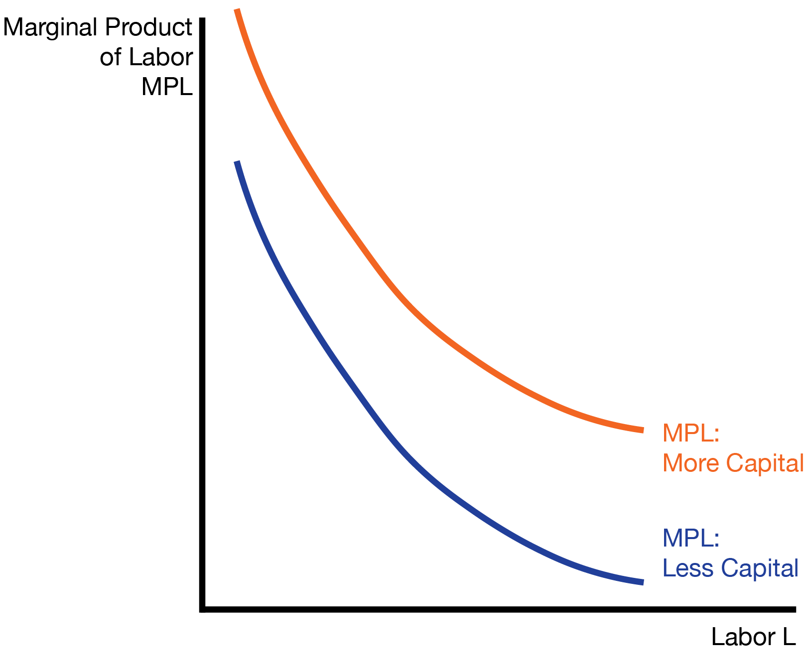
We will assume that the marginal productivity of capital (MPK) is increasing in labor and the marginal productivity of labor (MPL) is increasing in capital. The intuition is that with more labor workers, each unit of capital (each machine) is more productive. Equivalently, with more capital (machines or tools), each worker is more productive.
Finally, capital is paid the rental rate \(R\), and labor is paid the wage \(W\).
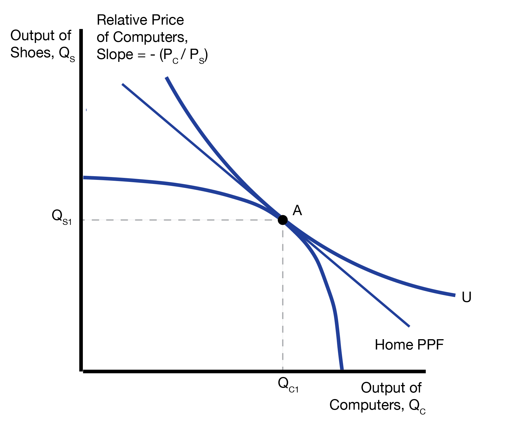
3.3 Autarky Equilibrium
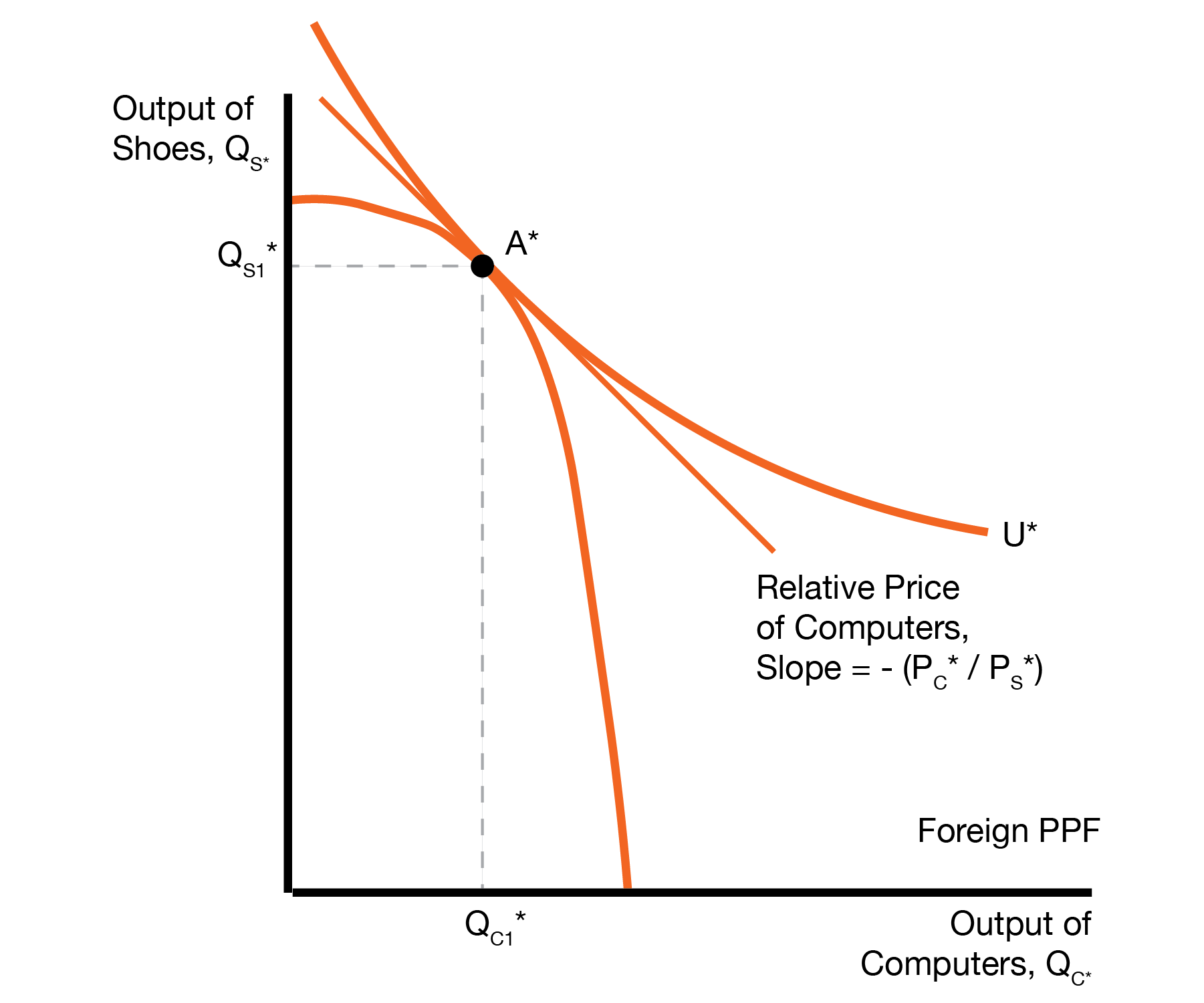
The autarky equilibria for Home and Foreign are given below. As with the Ricardian model, the equilibrium is determined by two things: what we can make (the PPF), and what we want (our indifference curves). In this case, we have a curved or bowed out PPF. This occurs because the marginal productivity of capital and labor changes, whereas the ricardian model features constant marginal productivities.
We will assume the autarky relative price of computers in Home is lower than in Foreign, \((P_C/P_S)^A < (P_C^*/P_S^*)^A\). The intuition is that Home is capital abundant, and computers are capital intensive, so it is easy for Home to produce computers. Because it’s easy to make computers, they are cheap in Home relative to Foreign. As a result, computers are ‘relatively’ cheap in Home.
3.4 Trade Equilibrium
We now allow Home and Foreign to trade at a world relative price of \((P_C / P_S)^W\). We start by considering the Home Export Supply Curve. At the autarky price of \((P_C / P_S)^A\), home doesn’t have any incentive to export, so the quantity of exports is zero. As the world price increases above the autarky price, Home computer makers can get more money abroad, so they start to export computers. This results in an increasing Home export supply curve. We wimilarly derive the Foreign import demand curve.
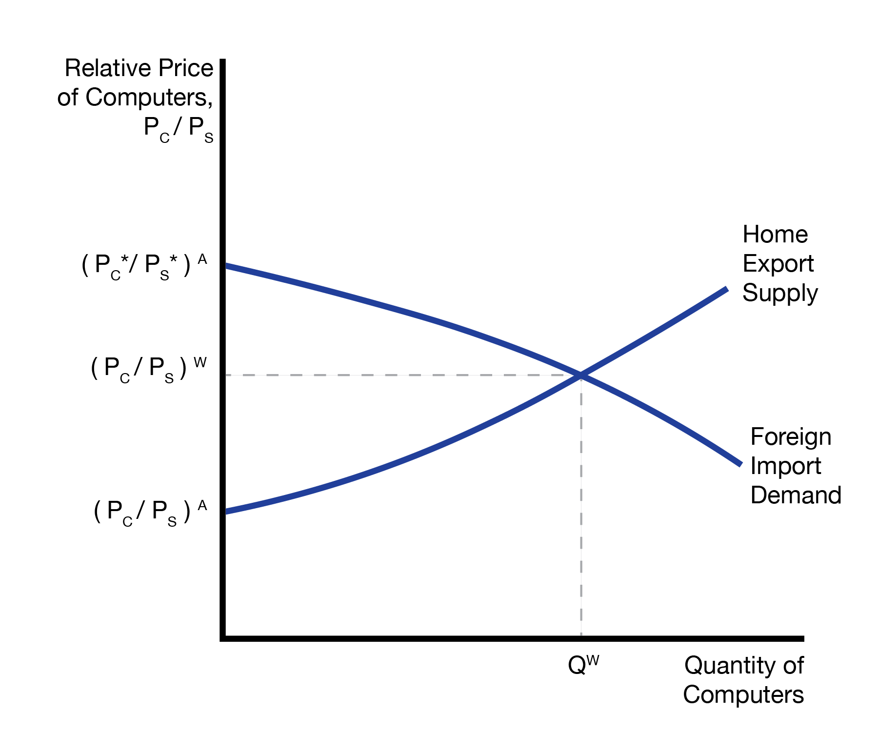
The trade market clears when Home exports of computers equals Foreign imports of computers. This provides the equilibrium trade price \((P_C / P_S)^W\) which is above the autarky price \((P_C / P_S)^A\).
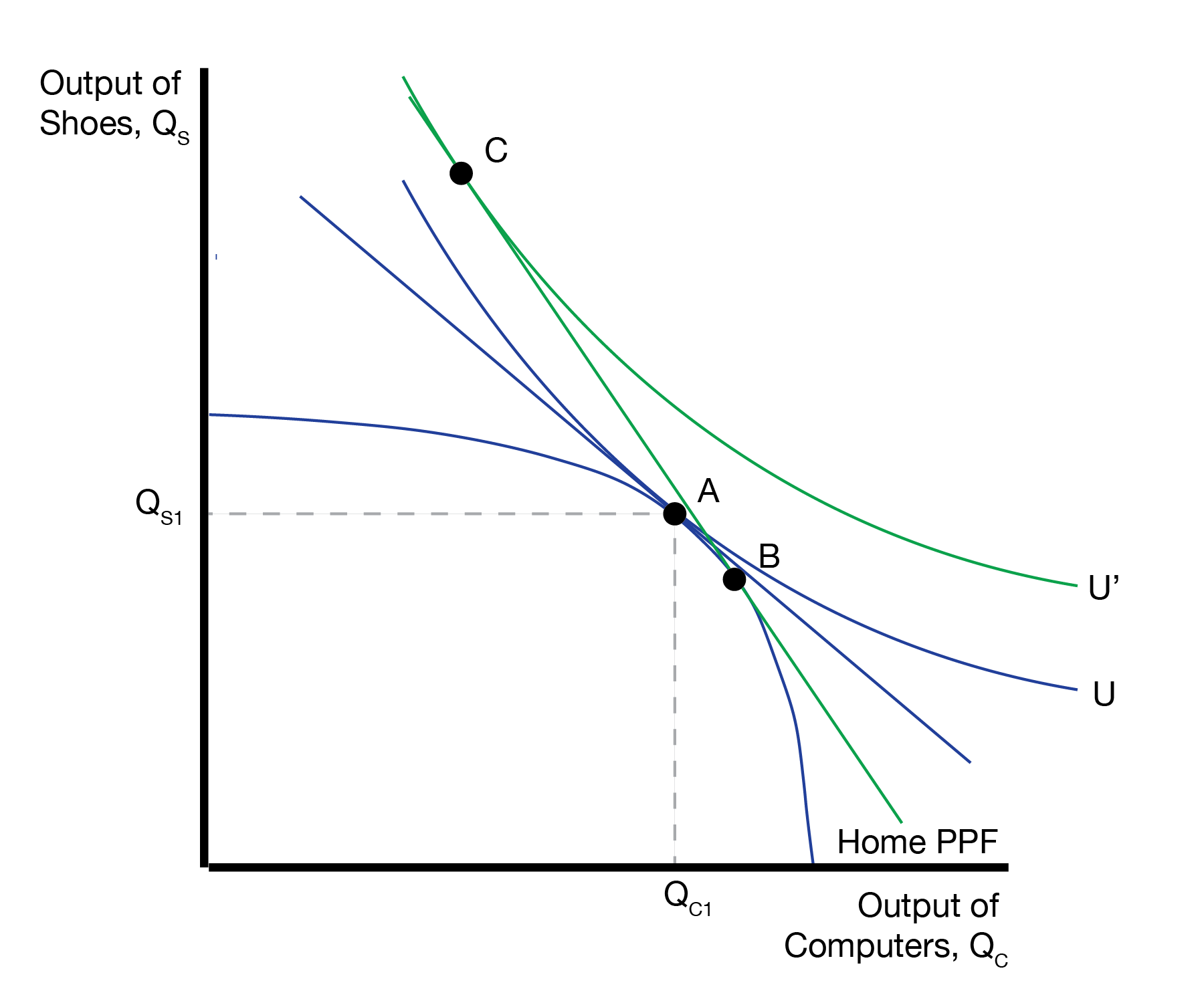
Given the new trade price, Home and Foreign now have to make the same choices they had to make once trade was introduced in the Ricardian. First, they decide where to produce, denoted by point \(B\) on the PPF. Second, they decide where to consume, denoted by point \(C\) on the trading curve.
The optimal production point is where the PPF is tangent to the trading curve, which has slope given by the relative price of computers to shoes \((P_C / P_S)^W\). Given this production point, households trade along the trading curve to their optimal consumption point \(C\), which is also tangent to the trading curve. Because the new indifference curve \(U'\) is higher than the autarky indifference curve \(U\), households are better off with trade. In this case, Home will export computers and import shoes.
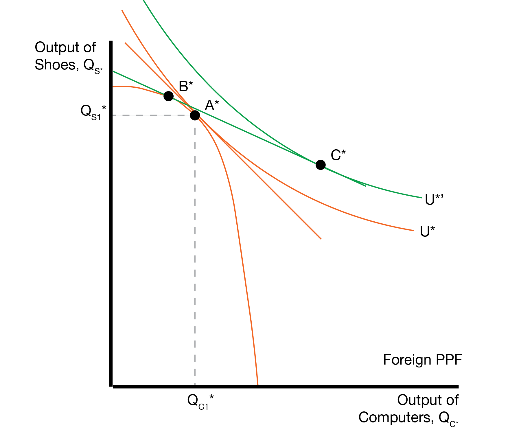
Foreign makes similar choices, producing at point \(B^*\) and consuming at point \(C^*\).
3.5 Winners and Losers
We now visit our two factors of production to see who wins and who possibly loses from trade.
Recall that capital earns rental rate \(R\). Each industry hires capital until the cost of capital \(R\) equals the marginal revenue product of capital. This provides two equations: \[ \begin{aligned} R &= P_C \times MPK_C \\ R &= P_S \times MPK_S. \end{aligned} \] We can then compute how many computers and shoes capital can purchase as \[ \begin{aligned} \text{Number of computers} = R / P_C &= MPK_C \\ \text{Number of shoes} = R / P_S &= MPK_S \end{aligned} \] It’s therefore sufficient to know how \(MPK_C\) and \(MPK_S\) change.
Similarly, labor earns wage \(W\). We can solve for the number of computers and shoes labor can purchase as \[ \begin{aligned} \text{Number of computers} = W / P_C &= MPL_C \\ \text{Number of shoes} = W / P_S &= MPL_S, \end{aligned} \] so we similarly need to know \(MPL_C\) and \(MPL_S\).
We will start by decomposing the total ‘relative’ labor supply as \[ \frac{\bar{L}}{\bar{K}} = \frac{\bar{L}_C + \bar{L}_S}{\bar{K}} = \frac{L_C}{K_C} \times \frac{K_C}{\bar{K}} + \frac{L_S}{K_S} \times \frac{K_S}{\bar{K}} \]
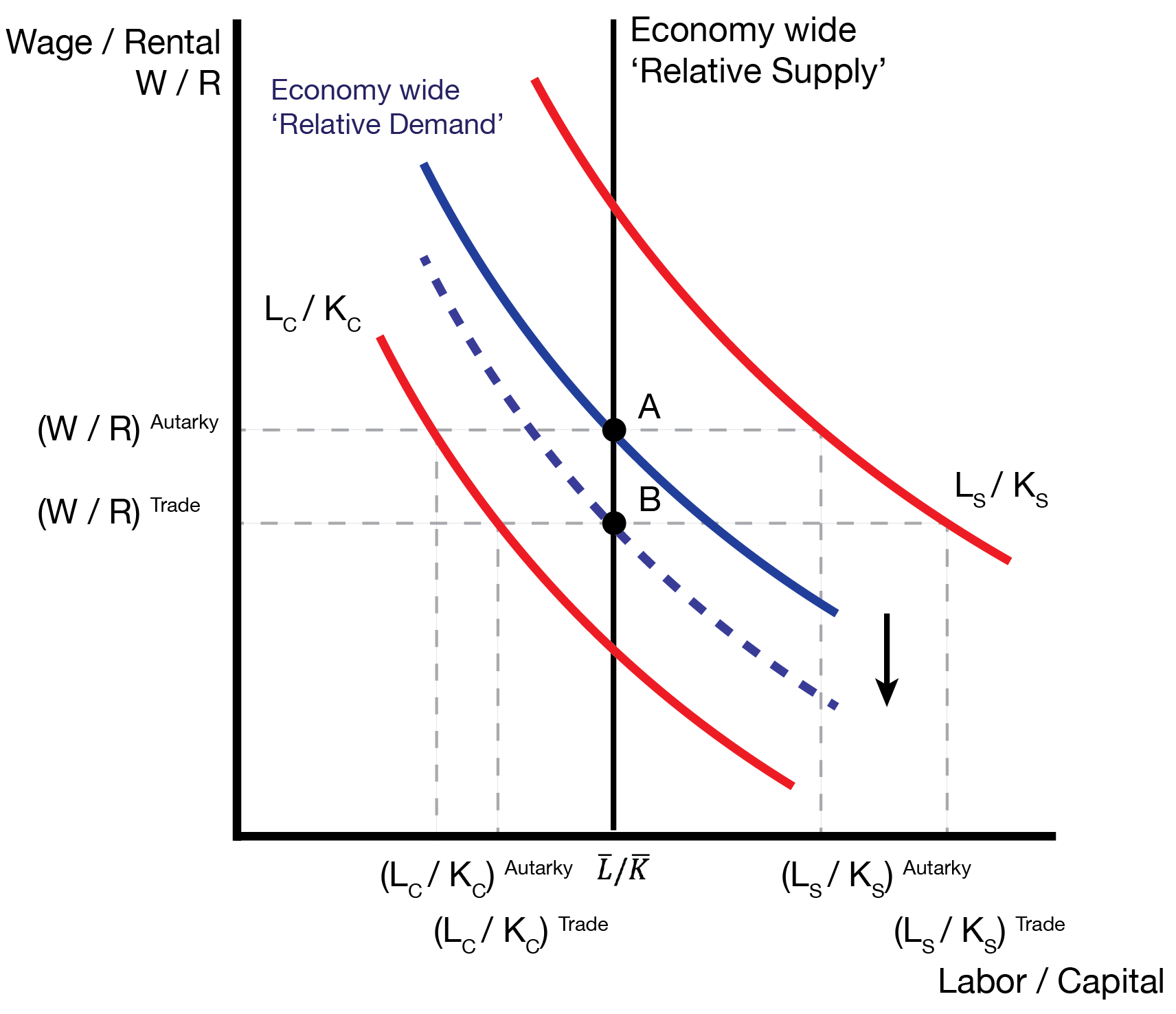
After trade we start producing more computers and less shoes, so \(K_C\) has increased and \(K_S\) has decreased. We can interpret this as a downward shift in the relative demand curve of the economy. Further, we can see the labor to capital ratio has increased in each indudstry.
We therefore have an increase in the marginal productivity of capital in computers \(MPK_C\) and shoes \(MPK_S\). Because capital owners can buy more computers and more shoes, they are better off after trade. In contrast, we have a decrease in the marginal productivity of labor in computers \(MPL_C\) and shoes \(MPL_S\). Because labor can buy less computers and shoes, they are worse off after trade.
We summarize the welfare effects of trade on the two factors of production in the following table.
| P of Capital Intensive Good Increases | P of Labor Intensive Good Increases | |
|---|---|---|
| Capital | Better off | Worse off |
| Labor | Worse off | Better off |
This result is called the Stolper-Samuelson Theorem, which states which factor will win or lose from international trade.
The intuition is that you want to be essential (intensive) to the industry that catches a high price. When trade occurs, the price of computers increases. Capital is essential (intensive) to making computers, so capital owners become well off. Similarly, the price of shoes decreases. This lowers the demand for labor, which is essential (intensive) to shoes. As a result, labor is worse off.
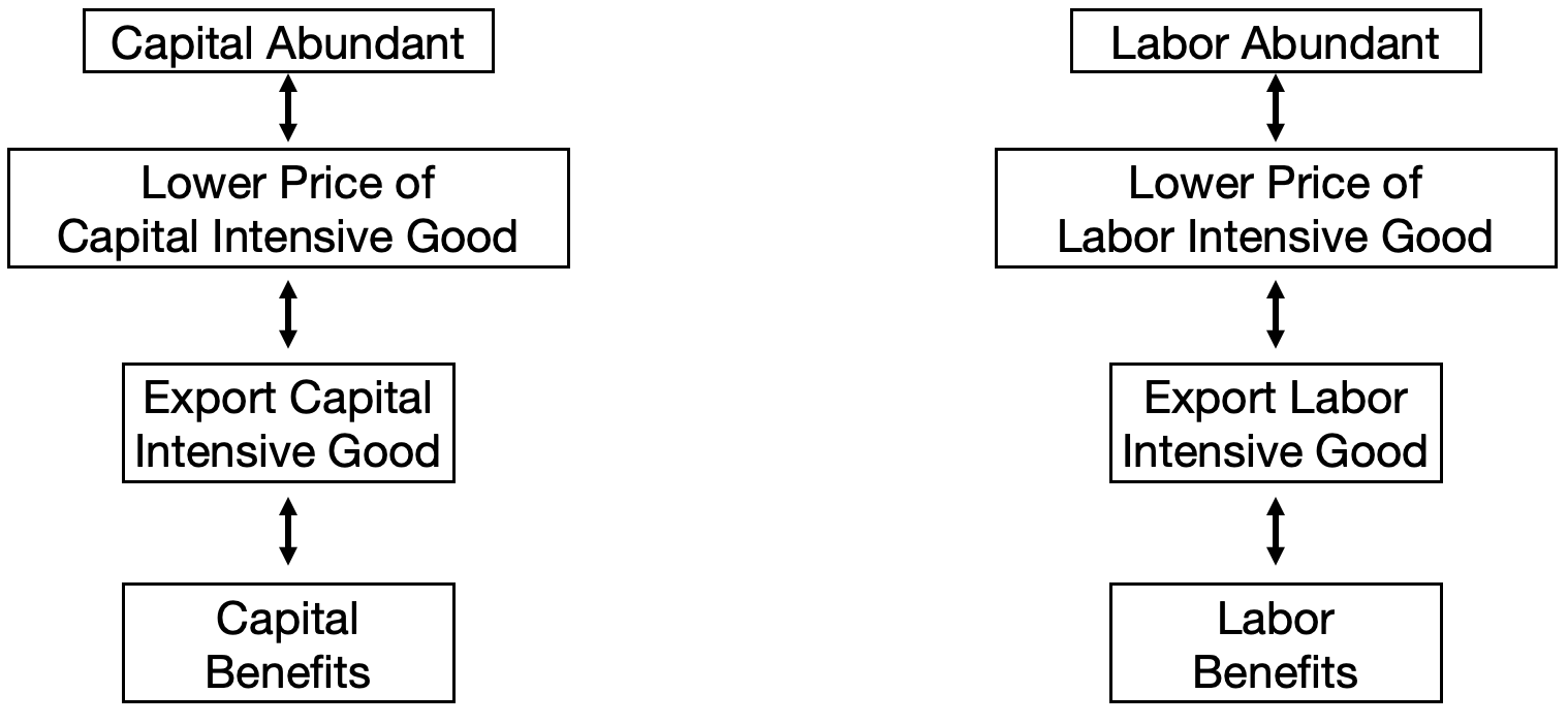
The trade patterns are given by the following table.
| Abundancy | Export Pattern | Import Pattern |
|---|---|---|
| Capital Abundant | Export Capital Intensive Good | Import Labor Intensive Good |
| Labor Abundant | Export Labor Intensive Good | Import Capital Intensive Good |
Countries export the good which they are ‘abundant’ in.
The effects on welfare are given as follows:
| Abundancy | Benefits from Trade | Hurt by Trade |
|---|---|---|
| Capital Abundant | Capital | Labor |
| Labor Abundant | Labor | Capital |
The factor that is abundant benefits from trade because it can work in the exporting industry that fetches a higher price on the world market.
3.6 Conclusion
- We’ve developed our trade equilibrium for the Heckscher-Ohlin Model
- The most important finding is the Stolper-Samuelson Theorem
- An increase in the relative price of a good will increase the real earnings of the factor used intensively in that good
- E.g. the factor that benefits is the factor used intensively in the exporting sector
- The Heckscher-Ohlin Model has a different motivation for trade
- Different countries have different endowments of capital and labor