6 Exchange Rates: Short Run
Objectives
- Understand price stickiness in the short run
- Clear the short run money market
- Solve for equilibrium exchange rate in the foreign exchange (FX) market
- Solve for the equilibrium interest rate in the money market
- Compute short and long run responses to temporary and permanent shocks
- Understand fixed vs floating exchange rate regimes
- Understand the trilemma (impossible trinity)
6.1 Introduction: Short and Long Run
In the previous section, we developed the long-run model of the money market and exchange rate. In the long run, we allow the price level \(P\) to adjust to clear the money market, which gives us the exchange rate \(E\). In the short run, this is problematic. Prices are ‘sticky’ and typically don’t change overnight. How do we fix this?
In this section, we will introduce a new ‘price’: the interest rate.
| Clears Money Market | ‘Fixed’ | |
|---|---|---|
| Long Run | \(P\) | \(i_{US}\) |
| Short Run | \(i_{US}\) | \(P\) |
6.2 The Money Market
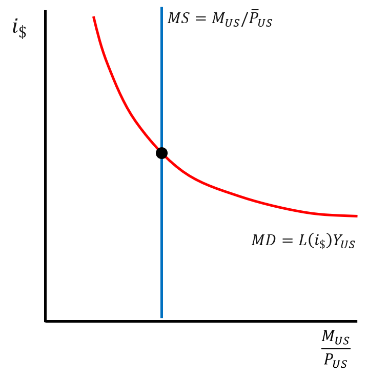
6.2.1 Shocks
| Shock | Nominal Interest Rate \(i_\$\) | Real Money \(M_{US}/P_{US}\) |
|---|---|---|
| \(M_{US} \uparrow\) | \(\color{red}{i_\$ \downarrow}\) | \(\color{green}{\frac{M_{US}}{P_{US}} \uparrow}\) |
| \(M_{US} \downarrow\) | \(\color{green}{i_\$ \uparrow}\) | \(\color{red}{\frac{M_{US}}{P_{US}} \downarrow}\) |
| \(Y_{US} \uparrow\) | \(\color{green}{i_\$ \uparrow}\) | No effect |
| \(Y_{US} \downarrow\) | \(\color{red}{i_\$ \downarrow}\) | No effect |
6.3 The Exchange Rate Market
\[ i_{USD} = i_{EUR} + \frac{E^{e}_{USD/EUR}}{E_{USD/EUR}} - 1 \]
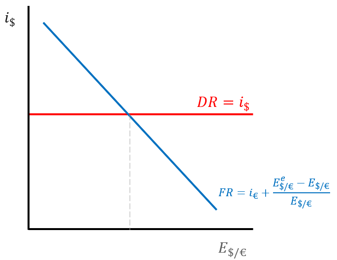
6.3.1 Shocks
| Shift | Exchange Rate EUSD/EUR |
|---|---|
| iUSD ↑ | Decrease ↓ |
| iUSD ↓ | Increase ↑ |
| iEUR ↑ | Increase ↑ |
| iEUR ↓ | Decrease ↓ |
| EeUSD/EUR ↑ | Increase ↑ |
| EeUSD/EUR ↓ | Decrease ↓ |
6.4 Connecting the Markets
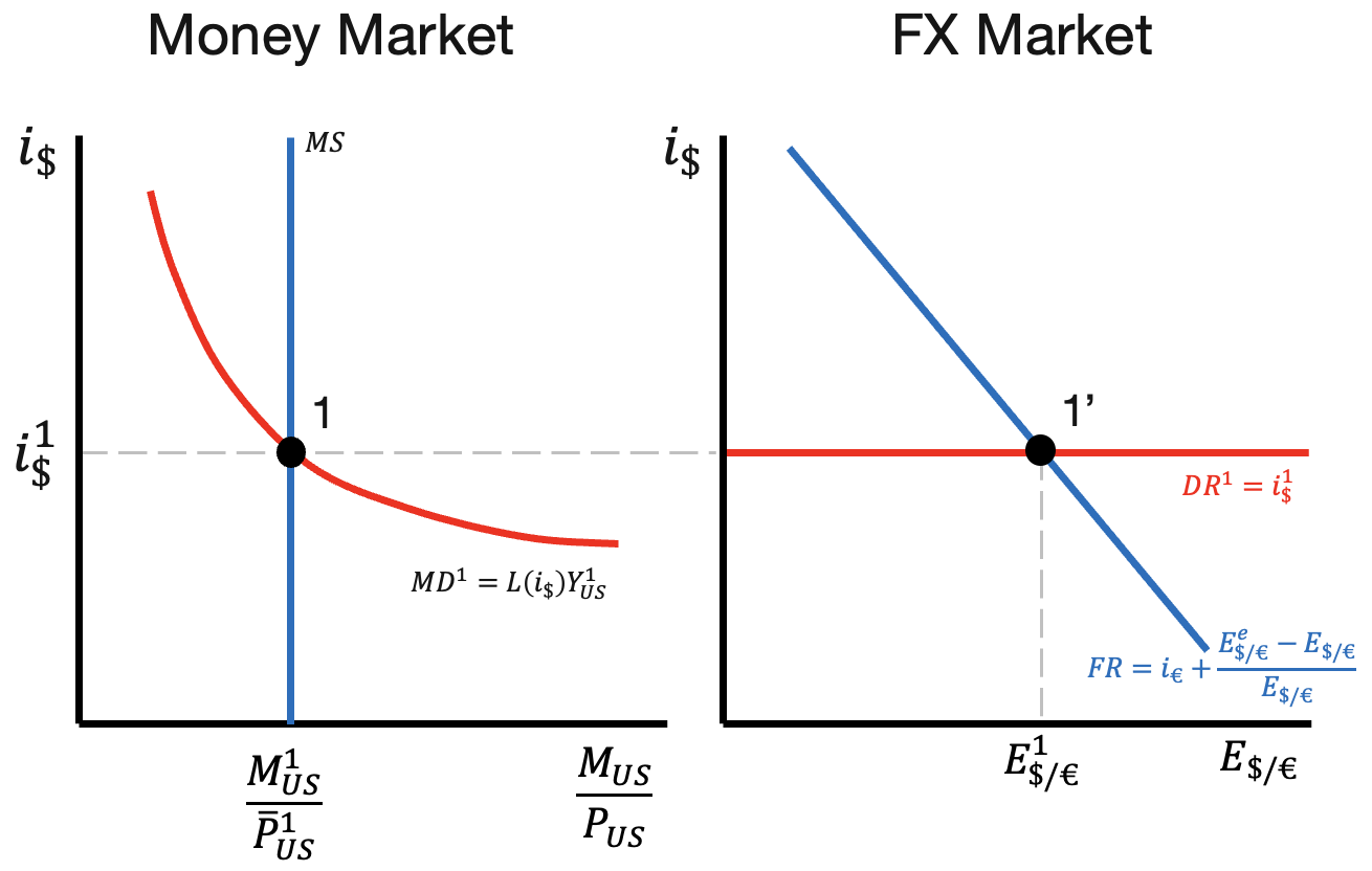
We now connect the money market and foreign exchange market. The two markets are connected through the U.S. interest rate \(i_{USD}\), which is an endogenous ‘outcome’ of the money market and an exogenous ‘input’ of the foreign exchange market. From this perspective, we can view the money market as ‘upstream’ of the foreign exchange market. We first solve the money market, so we know what interest rate to plug into the foreign exchange market.
6.4.1 Increase in Money Supply
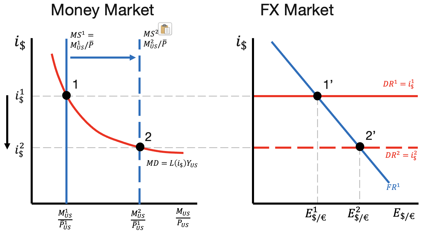
We now consider an increase in the money supply \(M_{US}\). This causes a rightward shift in the money supply \(M/P\) curve. Note that the money demand \(L(i) Y\) curve is unchanged because it doesn’t depend on \(M\). The increase in money supply produces a decrease in the equilibrium interest rate.
We now carry the interest rate decrease to the exchange rate market. The lower interest rate causes a depreciation of the dollar.
6.4.2 Increase in Real Income
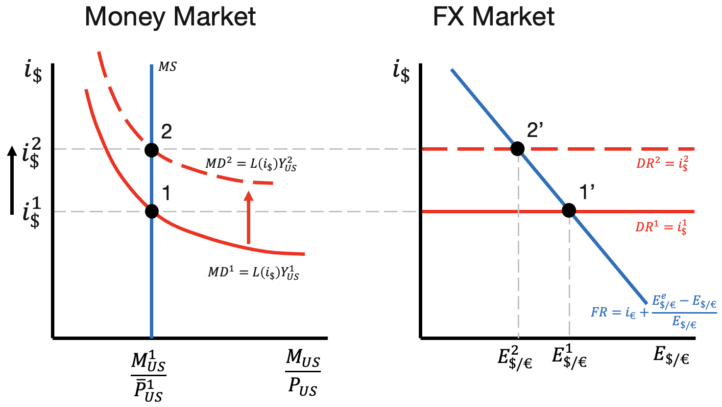
We now consider an increase in U.S. real income \(Y_{US}\). The increase in income \(Y\) produces an increase in the real money demand curve \(L(i) Y\). The money supply curve \(M/P\) is unchanged. The increase in real income produces an increase in the equilibrium interest rate.
We now carry the interest rate increase to the exchange rate market. The higher interest rate causes an appreciation of the dollar.
6.4.3 Foreign Money Supply Increase
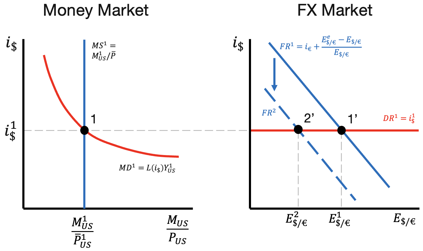
We now consider an increase in the foreign money supply \(M_{EUR}\). The increase in foreign money supply has no effect on the U.S. domestic money market, so the U.S. interest rate is unchanged. As a result, we carry the same original interest rate \(i_{USD}^1\) to the exchange rate market.
Within the European money market, the increase in money supply causes a decrease in the European interest rate \(i_{EUR}\). As a result, the \(FR\) curve shifts down, which causes an appreciation of the dollar.
6.5 Policy Objectives and the Trilemma
The trilemma states that a country cannot simultaneously achieve all three policy objectives of fixed exchange rates, international capital mobility, and monetary policy autonomy.
Note that if we have objectives 1 and 2, then we must have \(i_{USD} = i_{EUR}\), which violates objective 3.
If we have objectives 1 and 3, then we must have \(i_{USD} \neq i_{EUR}\), which violates objective 2.
Finally, if we have objectives 2 and 3, then we must have \(E_{USD/EUR}^e \neq E_{USD/EUR}\), which violates objective 1.
6.6 Conclusion
This section introduces the short-run model of exchange rates. We develop the money market, which is cleared by the interest rate \(i\) instead of the price level \(P\). We then develop the foreign exchange market, which determines the exchange rate \(E\).
The money and foreign exchange markets are connected through the interest rate \(i\), which is an endogenous outcome of the money market and an exogenous input in the foreign exchange market. When we study the responses of the economy to shifts or shocks, we first solve the money market to find the new equilibrium interest rate, and then carry that interest rate to the foreign exchange market to find the new equilibrium exchange rate.
Finally, we introduce the concept of the trilemma, which states that a country cannot simultaneously achieve all three policy objectives of fixed exchange rates, international capital mobility, and monetary policy autonomy.