5 Exchange Rates: Long Run
Objectives
- Compute the relative price of a good in two different countries (Law of One Price)
- Compute the relative price of a basket of goods in two different countries (Absolute Purchasing Power Parity)
- Know the relationship between inflation and exchange rate fluctuations (Relative Purchasing Power Parity)
- Build long-run equilibrium in the exchange rate model
- Map effects of changes in monetary policy and output growth on exchange rate and inflation
5.1 Introduction
Until now, we’ve taken the exchange rate as given, just as we take the price of bread as given at the market. We still want to know what determines the equilibrium exchange rate that we observe, just as we want to know what determines the price of bread. This section will provide structure so that we understand what determines the exchange rate. This will allow us to understand the current value of the exchange rate and make predictions about how it will change in the future.
5.2 Purchasing Power Parity
We start with the basic definition of the exchange rate:
The nominal exchange rate states how much it costs to buy another country’s currency. We will now consider how much it costs to buy another country’s goods rather than currency. We’ll consider a generic good \(g=\text{apple}\). It costs \(P_{EUR}^g\) Euros to buy a European apple. To have that many Euros, we need \(E_{USD/EUR} P_{EUR}^g\) dollars. The law of one price holds when the price of a U.S. apple in dollars is the same as a European apple in dollars.
Rather than focusing on a single good, we’re going to focus on all goods, which we average as a basket. In this case, \(P_{EUR}\) is the price of a basket in Europe, and \(P_{USD}\) is the price of a basket in the United States (this is commonly referred to as the price level). We will now develop the real exchange rate: how many U.S. baskets we give up for a European basket.
We start with the price of a European basket: \(P_{EUR}\) Euros. To obtain that many Euros, we need \(E_{USD/EUR} \times P_{EUR}\) Dollars. With \(E_{USD/EUR} \times P_{EUR}\) Dollars, we could have bought \(\frac{E_{USD/EUR} \times P_{EUR}}{P_{USD}}\) U.S. baskets.
We will consider the special case when \(q_{USD/EUR} = 1\). In this case, it costs 1 U.S. basket to buy 1 European basket. From \(q_{USD/EUR} = 1\), we can derive \(E_{USD/EUR} = \frac{P_{USD}}{P_{EUR}}\), which we call absolute purchasing power parity.
This has the sharp interpretation that the tradeoff of real baskets is the same as the tradeoff of nominal currencies.
Just as with the nominal exchange rate, we call an increase in the real exchange rate a real depreciation and a decrease a real appreciation.
| \(q_{USD/EUR}\) | Increase ↑ | Decrease ↓ |
|---|---|---|
| U.S. | Real depreciation | Real appreciation |
| Intuition | We give up more U.S. baskets for a single European basket | We give up less U.S. baskets for a single European basket |
We now examine a different form of purchasing power parity, relative purchasing power parity. Relative purchasing power parity is simply the relationship we see over time if absolute purchasing power parity holds. First solve \[ E_{USD/EUR} = \frac{P_{USD}}{P_{EUR}}. \]
We then apply the growth rate transformation to both sides of the equation. In this case, the growth rate of prices \(P_{USD}\) is inflation \(\pi_{USD}\) and likewise for \(EUR\).
5.3 Long-Run Model
We are now going to build a long run-model that describes the exchange rate. We have two goals for this model: why do we have the current exchange rate, and what drives changes in the exchange rate.
Until now, we’ve developed absolute and relative purchasing power parity, which state that the exchange rate depends on the price levels of each economy. But we wanted to know where the exchange rate (a price) originates, and purchasing power parity simply leads us to another price. We will therefore further develop the model to account for the price level of each country. To do this, we will start by developing a market for money which determines the price level.
5.3.1 Money Supply
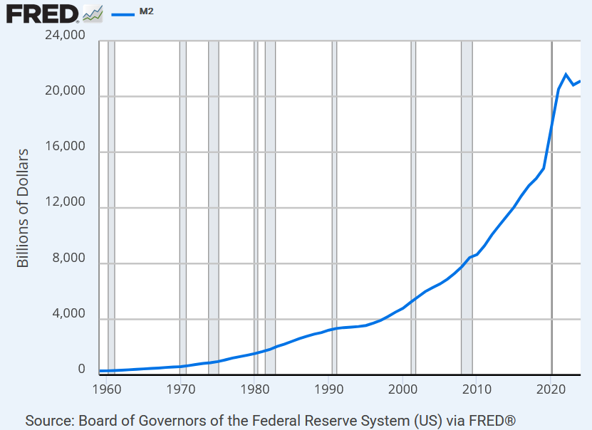
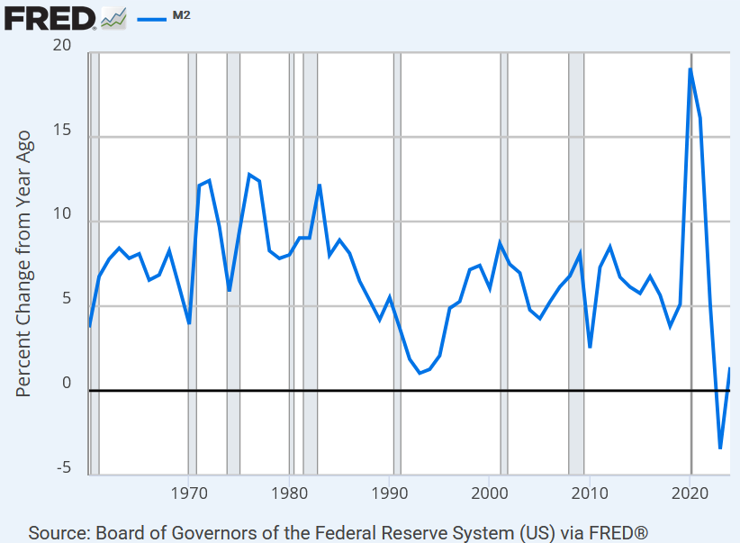
The money supply \(M\) is simply the sum of currency units available within a country. We assume the money supply is set by a nation’s central bank.
The following two figures show the money supply of the United States and its growth rate. As we can see, the growth rate transformation ‘scales down’ the money supply and makes its change comparable across time. As with the data, we will develop a similar ‘growth rate’ version of this model.
5.3.2 Money Demand
The supply of money is set by the central bank, so we now develop the demand for money.
We assume consumers have \(PY\) dollars of income and want to spend a fraction \(\bar L\) of that money. Consumers therefore need \(M^d = \bar L \times PY\) dollars in their wallets.
We can also solve for real money demand, how many baskets consumers purchase. In this case, consumers spend \(\bar L \times PY\) dollars. A basket costs \(P\), so they purchase \(\bar L \times Y\) baskets.
5.3.3 Money Market Equilibrium
Just as in the markets for cars or video game consoles, the money market clears when money supply equals money demand. In this case, the price level \(P\) adjusts to clear the market, just as the price of cars adjusts to clear the car market.
5.3.4 Simple Long Run Model - Growth Rate Form
We saw in the data that the growth rate transformation is useful for making changes comparable across time and across countries. We will therefore apply the growth rate transformation to our model. Applying the growth rate to both sides of the money market clearing condition, we obtain
\[ \mu_t = g_t + \pi_t, \]
where \(\mu_t\) is the growth rate of money \(M\), \(g_t\) is the growth rate of output \(Y\), and \(\pi_t\) is the growth rate of prices \(P\).
We now develop our model for how exchange rates evolve over time. Relative purchasing power parity implies \[ \frac{\Delta E_{\text{USD}/\text{EUR},t}}{E_{\text{USD}/\text{EUR},t}} = \pi_{US,t}-\pi_{EUR,t}. \]
From the money market clearing condition, we substitute \(\pi_{x,t} = \mu_{x,t} - g_{x,t}\), which provides
\[ \frac{\Delta E_{\text{USD}/\text{EUR},t}}{E_{\text{USD}/\text{EUR},t}} = \left( \mu_{US,t} - \mu_{EUR,t} \right) - \left( g_{US,t} - g_{EUR,t}\right) \]
Our model can therefore be expressed as two equations:
5.4 Long-Run Model: Shocks
We’ve solved for the money and exchange rate equilibria. We now want to understand how the equilibrium responds to shocks.
Shocks can come from the exogenous or ‘given’ variables of the model. In the money market, the exogenous variables are the growth rate of money \(\mu_t\) and the growth rate of output \(g_t\) for each country.
5.4.1 Increase in the Growth Rate of Money
We now consider the effects of an increase in the growth rate of the U.S. money supply. We model this as an increase in the money supply growth rate from \(\mu_{USD,t}\) to \(\mu_{USD,t} + \Delta \mu\).
\[ \begin{aligned} (\mu_{US,t} + {\color{red}\Delta \mu}) &= g_{US,t} + (\pi_{US,t} + {\color{red}?}) \\ \frac{\Delta E_{\text{USD}/\text{EUR},t}}{E_{\text{USD}/\text{EUR},t}} + {\color{red}?} &= \left( \mu_{US,t} + {\color{red}\Delta \mu} - \mu_{EUR,t} \right) - \left( g_{US,t} - g_{EUR,t}\right) \end{aligned} \]
How does this impact the equilibrium? Visiting the money market, we must now satisfy \(\mu_t + \Delta \mu = g_t + \pi_t\). Because the left-hand side has increased by \(\Delta \mu\), the right-hand side must also increase by \(\Delta \mu\). Because \(g_t\) is exogenous (taken as given), it must be that inflation \(\pi_t\) has increased by \(\Delta \mu\). The increase in money supply therefore produces an increase in inflation by the same amount.
We now visit the exchange rate market. We must satisfy the equation \[ \frac{\Delta E_{\text{USD}/\text{EUR},t}}{E_{\text{USD}/\text{EUR},t}} + {\color{red}?} = \left( \mu_{US,t} + {\color{red}\Delta \mu} - \mu_{EUR,t} \right) - \left( g_{US,t} - g_{EUR,t}\right). \]
Everything else on the right-hand side is exogenous (unchanged). Therefore, it must be that the growth rate of the exchange rate \(\Delta E / E\) increases by \(\Delta \mu\). The increase in the growth rate of the money supply therefore leads to an exchange rate depreciation.
| \(\mu_{USD,t}\) | Increases | Decreases |
|---|---|---|
| Inflation πUS,t | Increases | Decreases |
| Exchange Rate EUS/EUR,t | Increases (Depreciates) | Decreases (Appreciates) |
5.4.2 Increase in Home Income
We now consider the effects of an increase in home income. We will model this as an increase from \(g_{USD,t}\) to \(g_{USD,t} + \Delta g\).
\[ \begin{aligned} \mu_{US,t} &= (g_{US,t} + {\color{red}\Delta g}) + (\pi_{US,t} + {\color{red}?}) \\ \frac{\Delta E_{\text{USD}/\text{EUR},t}}{E_{\text{USD}/\text{EUR},t}} + {\color{red}?} &= \left( \mu_{US,t} - \mu_{EUR,t} \right) - \left( g_{US,t} + {\color{red}\Delta g} - g_{EUR,t}\right) \end{aligned} \]
How does this impact the equilibrium? In the money market equation, \(\mu\) is taken as given (unchanged), so only a change in \(\pi\) can restore equilibrium. Therefore, \(\pi\) must decrease by \(\Delta g\).
Within the exchange rate market, everything else on the right-hand side is exogenous (unchanged), so the growth rate of the exchange rate \(\Delta E / E\) must decrease by \(\Delta g\).
| \(g_{USD,t}\) | Increases | Decreases |
|---|---|---|
| Inflation πUS,t | Decreases | Increases |
| Exchange Rate EUSD/EUR,t | Decreases (Appreciates) | Increases (Depreciates) |
5.4.3 Application: Increase in Foreign Money Supply
We now consider the impact of an increase in Foreign’s money supply. We will model this as an increase from \(\mu_{EUR,t}\) to \(\mu_{EUR,t} + \Delta \mu\).
\[ \begin{aligned} \mu_{US,t} &= g_{US,t} + \pi_{US,t} \\ \frac{\Delta E_{\text{USD}/\text{EUR},t}}{E_{\text{USD}/\text{EUR},t}} + {\color{red}?} &= \left( \mu_{US,t} - (\mu_{EUR,t} + {\color{red} \Delta \mu_{EUR}}) \right) - \left( g_{US,t} - g_{EUR,t}\right) \end{aligned} \]
We first visit the U.S. money market, which must satisfy \(\mu_t = g_t + \pi_t\). Notice that because \(\mu_t\) and \(g_t\) are unchanged, the resulting inflation \(\pi_t\) is unchanged. Why is this? The U.S. has the same amount of money and goods, so U.S. prices don’t need to change in order to clear the U.S. money market.
Next, we visit the foreign exchange market. The market must satisfy \(\frac{\Delta E_{\text{USD}/\text{EUR},t}}{E_{\text{USD}/\text{EUR},t}} + {\color{red}?} = \left( \mu_{US,t} - (\mu_{EUR,t} + {\color{red} \Delta \mu_{EUR}} ) \right) - \left( g_{US,t} - g_{EUR,t}\right)\) , so \(\frac{\Delta E_{USD/EUR}}{E_{USD/EUR}}\) has decreased, or the dollar has appreciated. Why is this? The European money supply has increased, so Euros become less scarce and less valuable. U.S. dollars become relatively more scarce, so the Dollar appreciates.
The most uncomfortable part is that the shock impacts the exchange rate, but not U.S. inflation. But we see this every day when economies experience hyperinflations that aren’t inherited by the United States. The intuition is that the foreign money supply shock only impacts the exchange rate because the two economies link there. U.S. prices (and inflation) only need to clear the U.S. money market, so they don’t depend on the European money market.
| \(\mu_{EUR,t}\) | Increases | Decreases |
|---|---|---|
| Inflation πUS,t | Unchanged | Unchanged |
| Inflation πEUR,t | Increases | Decreases |
| Exchange Rate EUSD/EUR,t | Decreases (Dollar Appreciates) | Increases (Dollar Depreciates) |
6 Conclusion
We’ve examined the exchange rate and its evolution, just as we might study the price of cars or housing. This lecture develops a theory for the origin of the exchange rate: what sets its current level and how it changes over time. We first develop relative purchasing power parity, which shows that the exchange rate depends on the price level of each economy. We then develop the money market, which tells us the price level in each economy depends on their respective money supply.
This provides a long-run model which provides i) the price level and ii) the resulting exchange rate. Lastly, we examine the growth rate form of the model to study how exchange rates and prices change over time.