10 Labor
Objectives
- Understand origin of labor demand through marginal product and marginal reveune product of labor
- Identify labor demand shifters
- Identify labor supply shifters
- Solve for labor market equilibrium and map effects of supply/demand shifts
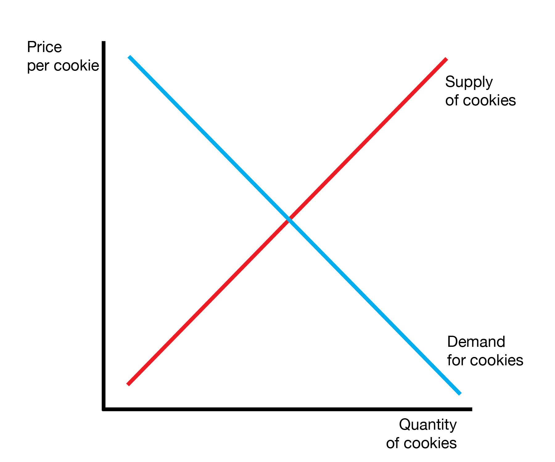
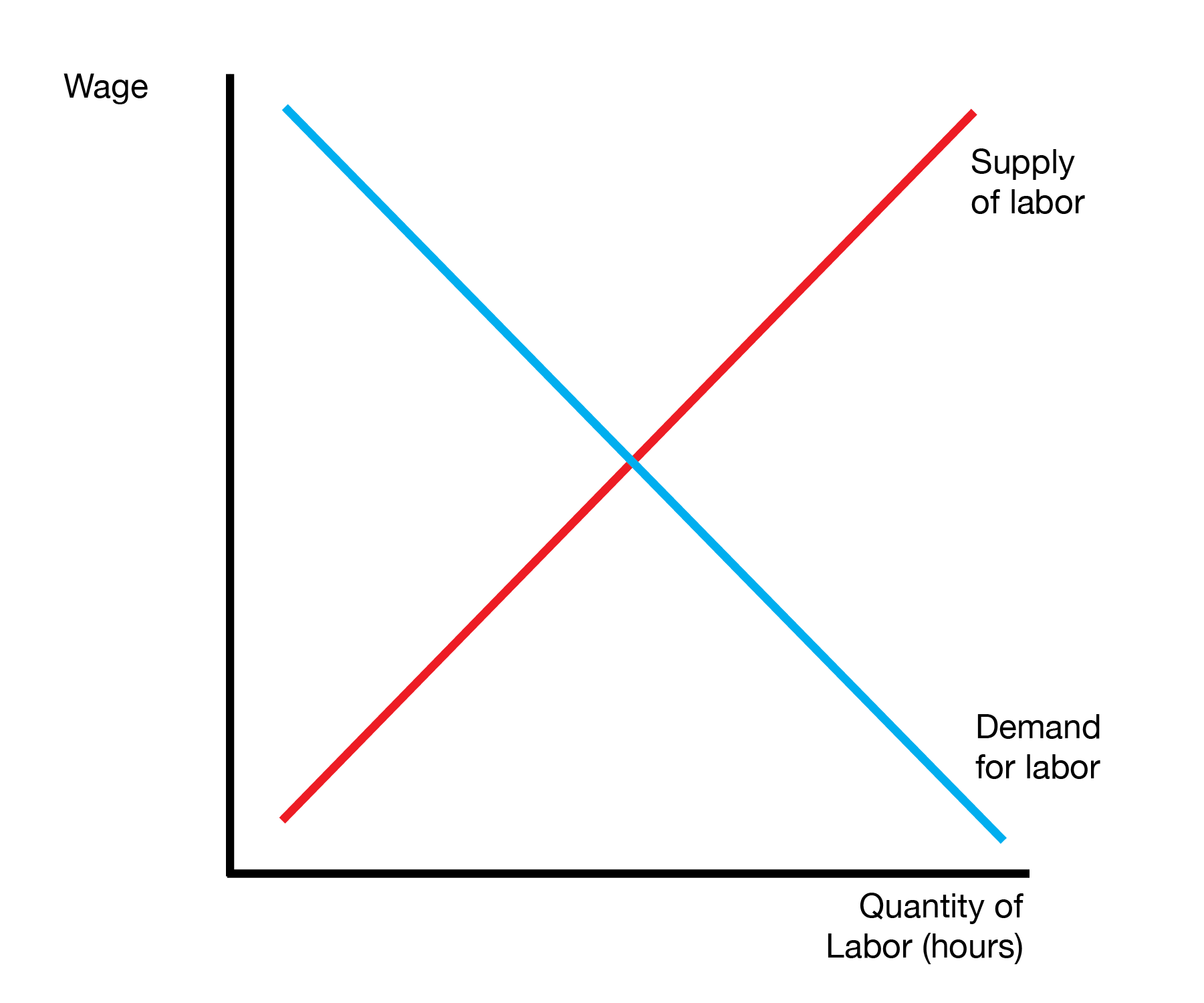
This section studies the labor market, or the market for work and employment. We will largely follow the structure we use in regular markets for goods such as jeans and cars. The quantity is either the amount of hours worked or number of people employed. The ‘price’ of labor is the wage, or how much each worker is paid. The only catch is that firms will now demand or consume labor, and workers will supply labor. This differs from our usual notion of the firm as a producer.
10.1 Demand for Labor
We start by developing our demand curve for labor. We begin by defining the marginal product of labor, the extra production that occurs from hiring an extra worker. Critically, we assume the marginal product of labor is decreasing. This has two interpretations. First, if we hire a worker they are most productive in the first hour, less productive in the second hour, and so on. Our second interpretation is if we are hiring many workers. We hire the most productive worker first, then the second most productive worker, then the third most productive worker, and so on. Either interpretation provides a downward sloping marginal productivity of labor.
The firm fundamentally cares about the money (revenue) each employee brings in, not just the product that they make. We multiply by the price to get the marginal revenue product of labor, the marginal revenue from hiring an additional worker.
Finally, the firm is ready to choose the number of workers to hire. We use marginal benefit-cost analysis. The marginal benefit of each employee is the revenue they bring in (marginal revenue product of labor). The marginal cost of each employee is the wage they must be paid.
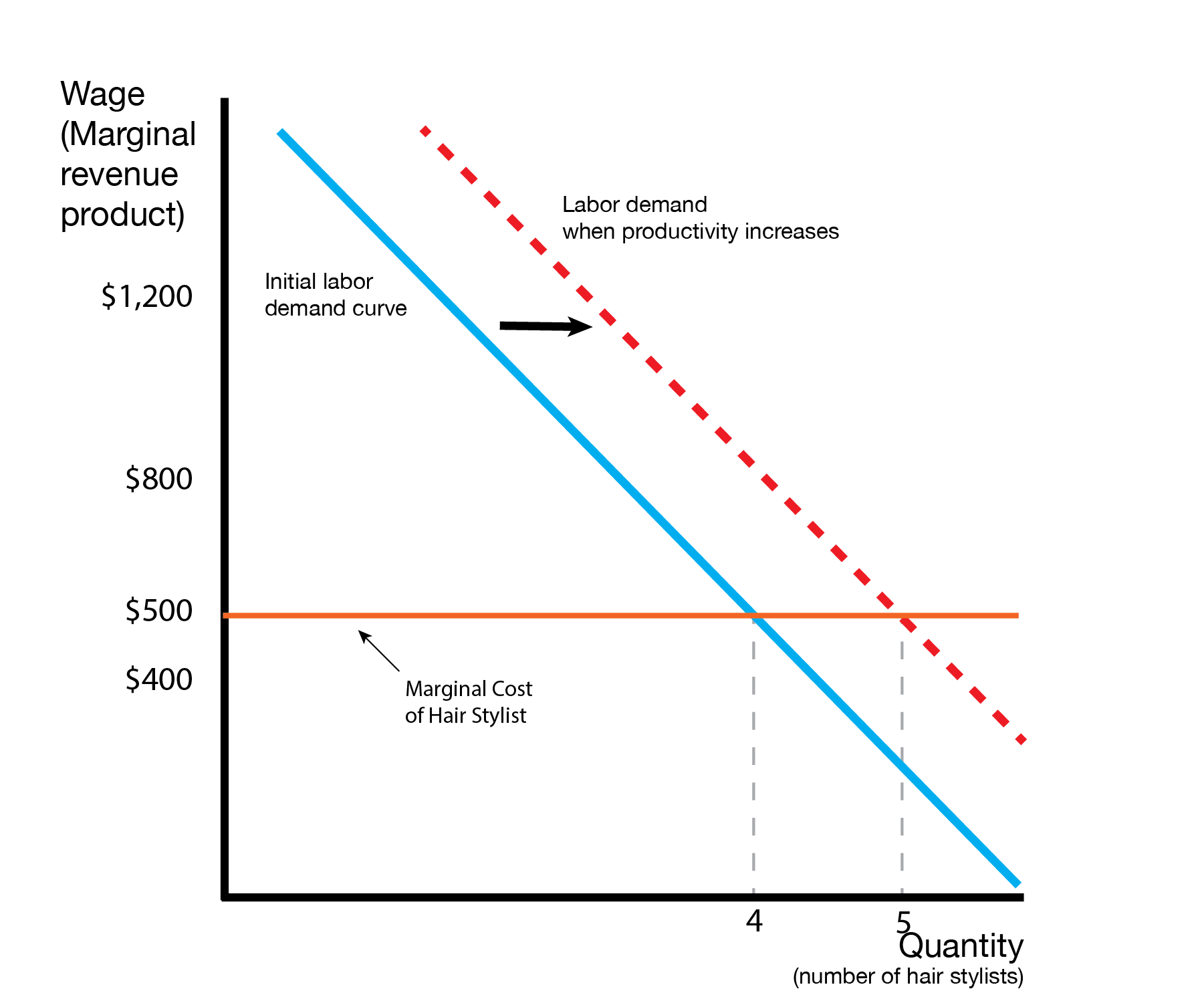
Consider the following table, which studies the number of hair stylists to hire. The first stylist brings in $800, and costs $500, so we hire them. We similarly hire the 2nd and 3rd hair stylist. The 4th hair stylist presents the edge case: they bring in $500 of revenue but cost $500. As before, we assume the firm follows through on the edge case and will hire the 4th hair stylist.
Should we hire the 5th stylist? They bring in $400 of revenue but cost $500. The firm will therefore only hire four stylists.
| Number of hair stylists | Marginal product (additional haircuts per week) | Marginal revenue product (Marginal product × $20 per haircut) = Marginal Benefit | Wage for a hair stylist = Marginal Cost |
|---|---|---|---|
| 1 | 40 | $800 | $500 |
| 2 | 35 | $700 | $500 |
| 3 | 30 | $600 | $500 |
| 4 | 25 | $500 | $500 |
| 5 | 20 | $400 | $500 |
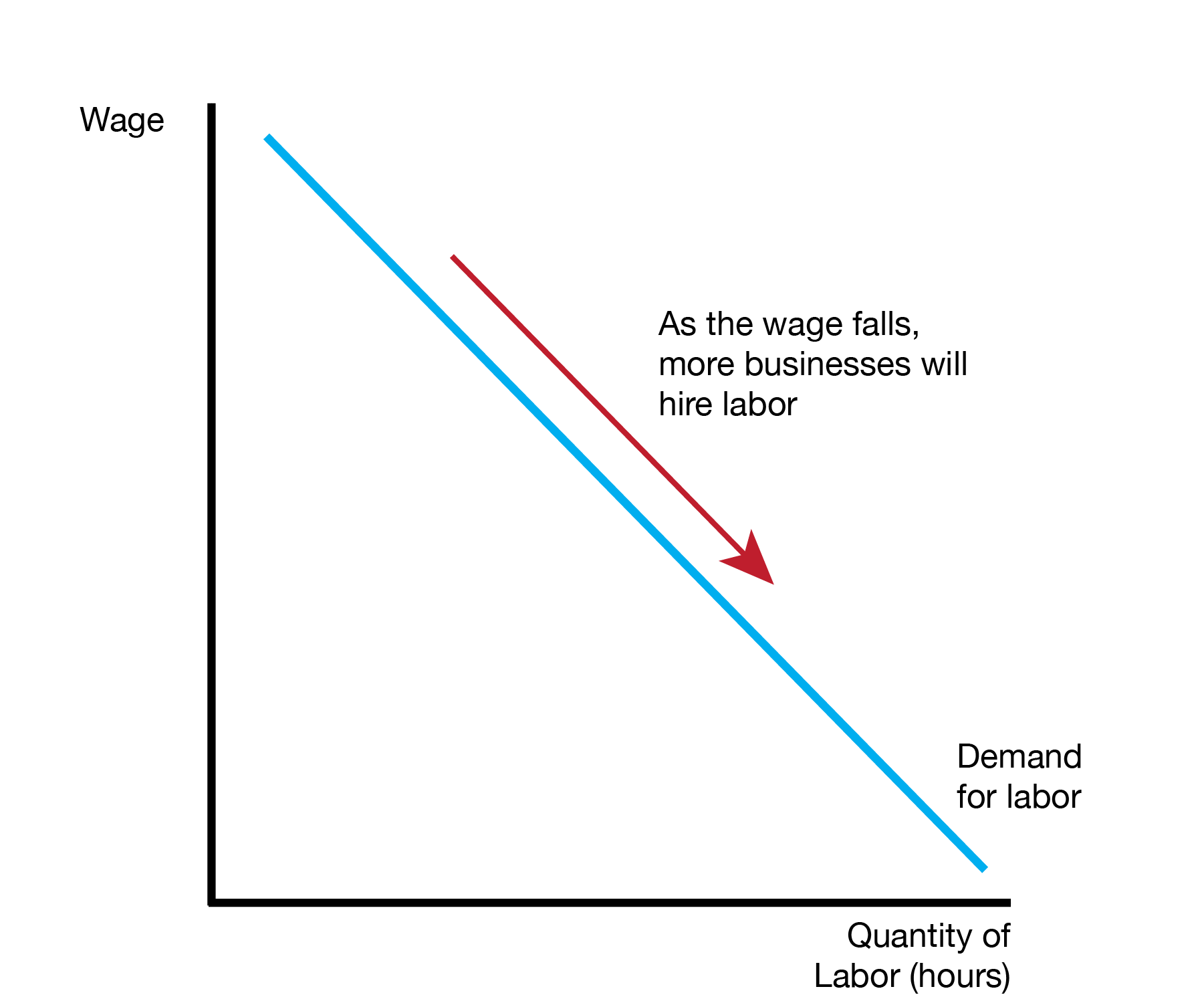
10.2 Movements along the Labor Demand Curve
The previous section develops the labor demand curve. Similar to the demand curve for goods such as jeans, a change in the price of labor (wage / income), will lead to changes in the quantity demanded of labor. We trace the change by simply moving up or down the labor demand curve.
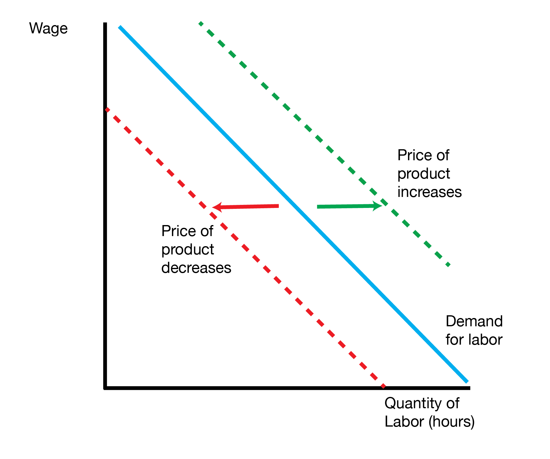
10.3 Labor Demand Shifters
We now introduce shifts to the labor demand curve. Labor demand shifts when something other than the price of labor (wage/income) changes.
The most prominent is the price of the underlying product the firm sells. If the price increases, the marginal revenue product of labor increase and the firm wants to hire more labor at every labor price (wage/income). Note this is a shifter because the price of something other than the price of labor is changing. Simiarly, if the price decreases, the marginal revenue product of labor decreases and the firm wants to hire less labor at every labor price (wage/income).
We now categorize labor demand shifters other than the price of the good sold by the firm. The first category is changes in the price of capital, where capital is the ‘machinery’ used to make products, like computers. If labor and capital are complements in production, an increase in the price of capital decreases demand for labor. In contrast, if labor and capital are substitutes in production, an increase in the price of capital increases demand for labor. Productivity or management improvements increase the marginal product of labor and hence the marginal revenue product of labor. Finally, an increase in nonwage benefits or subsidies decreases labor demand. This includes health insurance, paid sick leave, vacation days, etc. The key is that this is not the direct wage or income paid to employees, so it is a shifter.
| Labor Demand Shifter | Effect on Labor Demand |
|---|---|
| Increase in price of product | Increase |
| Increase in price of capital (complements) | Decrease |
| Increase in price of capital (substitutes) | Increase |
| Productivity/management improvements | Increase |
| Nonwage benefits/subsidies | Decrease |
10.3.1 Management and Productivity Gains
10.4 Labor Supply
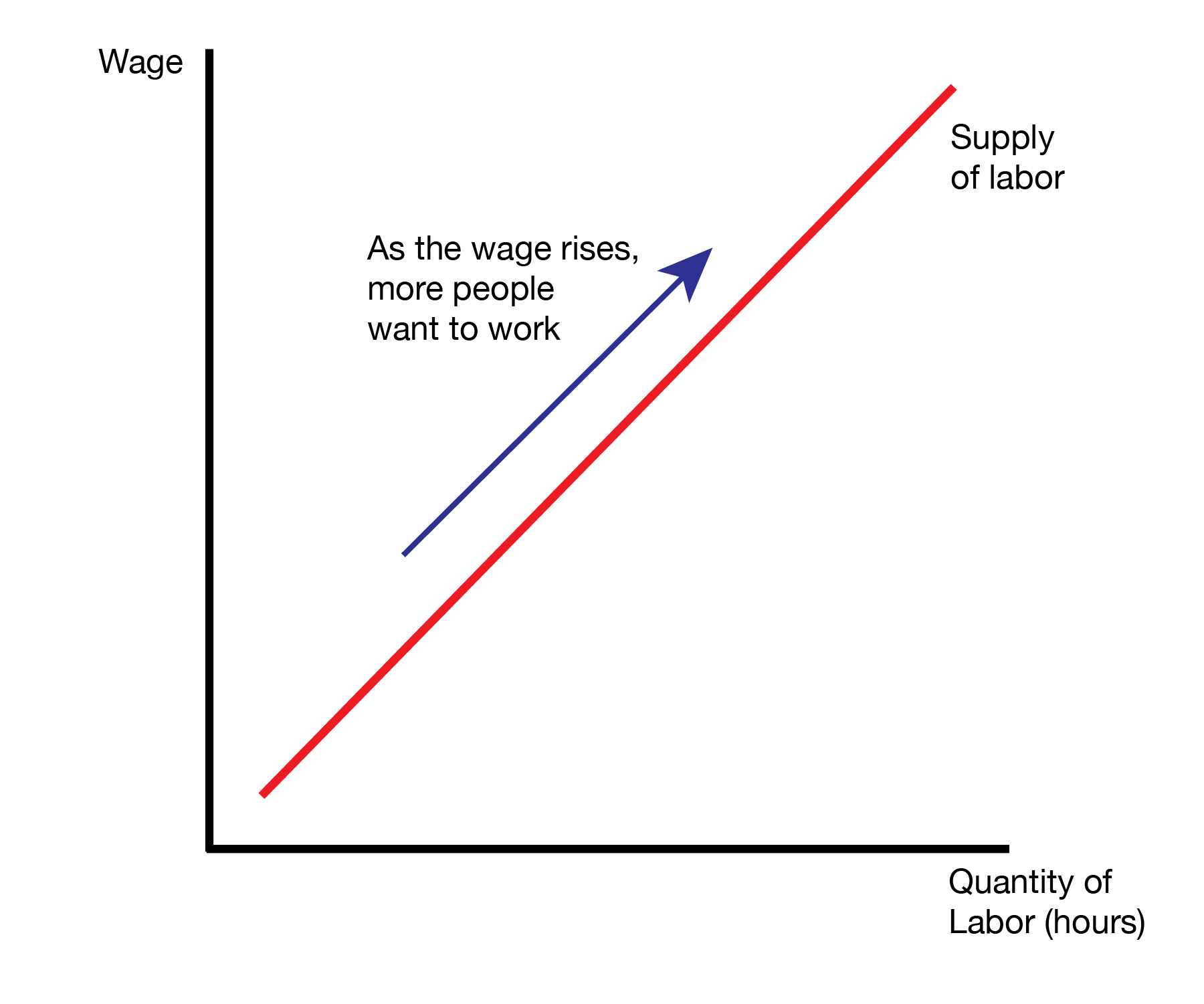
We now examine labor supply, which describes the realtionship between the wage (income) and how many workers want to work. The labor supply curve is increasing: as the wage increases, more workers want to work.
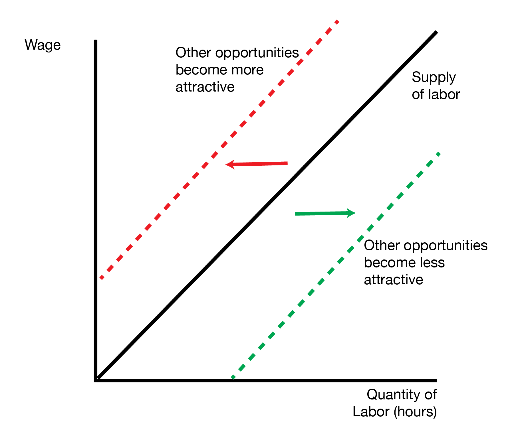
We now consider labor supply shifters, which are changes in things other than the wage. The first is wages in other occupations. An increase of the wage in other occupations makes workers more interested in the other occupation, which decreases supply. We can view workers are substituting across different occupations and supplying labor to the hire paying occupation, all else constant.
An increase in the number of workers increases the market supply of workers. An increase in the benefits of not working decreases the labor supply. Here we can view workers as choosing how to spend their time. As time ‘not working’ becomes more attractive, working becomes less attractive, so we have a decrease in supply. Opposite of the firm, an increase in nonwage benefits/subsidies makes working more attractive, which drives an increase in labor supply.
| Labor Supply Shifter | Effect on Labor Supply |
|---|---|
| Increase in wages in other occupations | Decrease |
| Increase in number of potential workers | Increase |
| Increase in benefits of not working | Decrease |
| Increase in nonwage benefits/subsidies | Increase |
10.5 Conclusion
- This lecture develops the labor market and labor market equilibrium
- Demand side: firm’s demand employees’ labor
- Supply side: employees supply labor
- We develop the equilibrium price (wage) and quantity (hours worked) of labor
- As before, we introduce labor supply and demand shifts that change the equilibrium