9 Market Power
Objectives
- Identify different market structures
- Perfect Competition
- Monopolistic Competition
- Oligopoly
- Monopoly
- Identify firm demand curve for different market structures
- Solve monopolist’s problem
- Compute marginal revenue curve
- Compute profit maximizing price and quantity and compare to competitive price and quantity
This section introduces market power, the ability of firms to command the price which they charge consumers. We first introduce four different market structures. Each market structure has a different level of market power. We then study the problem of the monopolist, who has complete market power.
9.1 Market Power
9.2 Perfect Competition
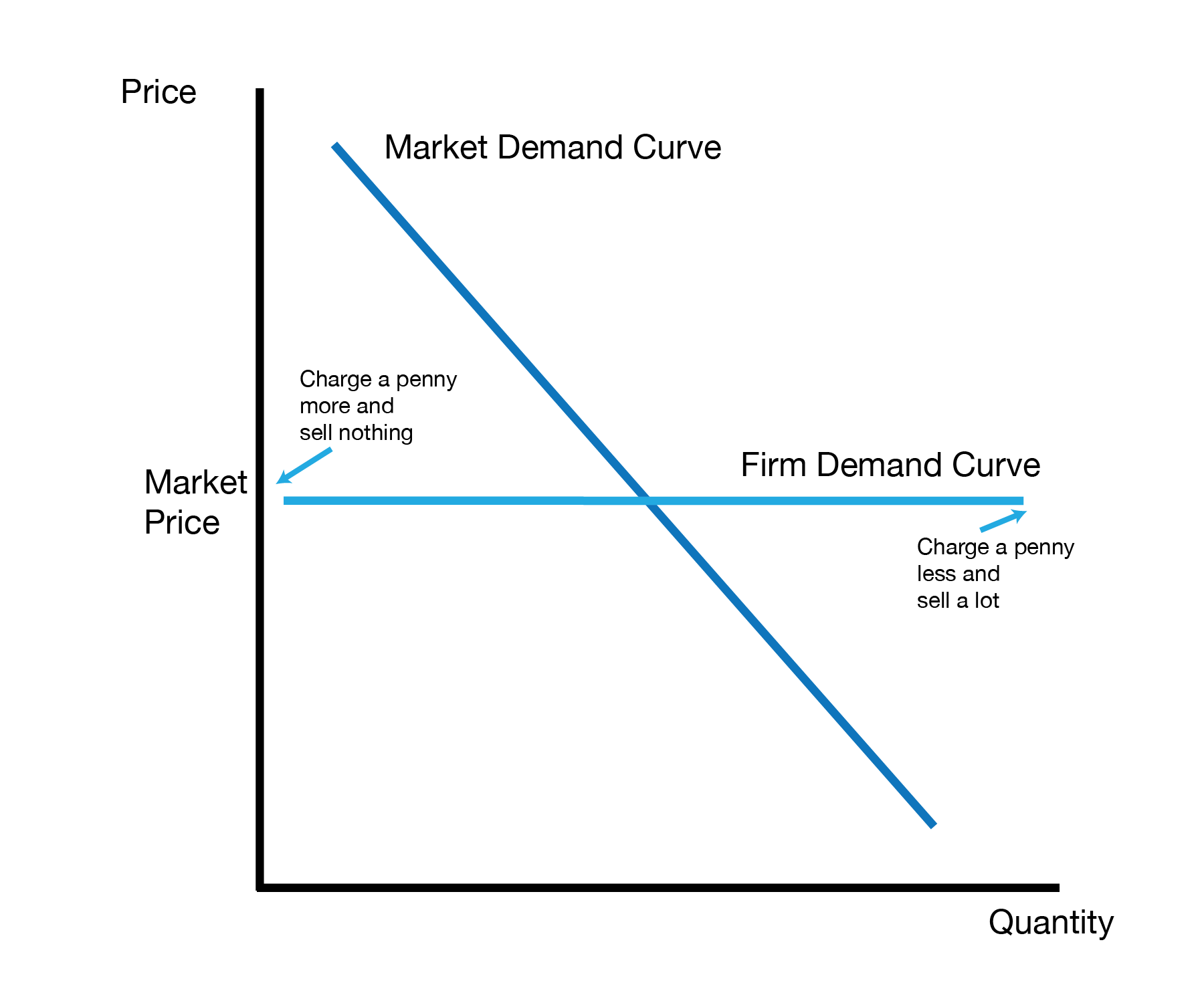
9.3 Imperfect Competition
We now study imperfect competition, in which firms have some market power but not absolute market power.
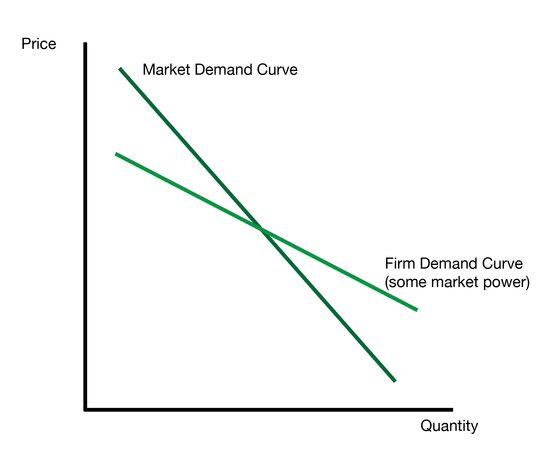
9.3.1 Oligopoly
Our first case of imperfect competition is oligopoly, where there are only a handful of large sellers in the market. Because there is a small number of sellers, they can ‘meet’ and coordinate the price they want to charge consumers. This differs from perfect competition, where if a small firm goes above the market price they lose all demand.
9.3.2 Monopolistic
Our next case is monopolistic competition. In this case there are many sellers, but they sell differentiated, or slightly different products. For instance, there are many different jeans. They differentiate themselves by different dyes, fabric cuts, and buttons. If a monopolistic seller increases their price, some consumers will leave and substitute to other products. However, the monopolistic seller has some ‘fans’ of their differentiated product. This allows them to keep some demand after raising their price.
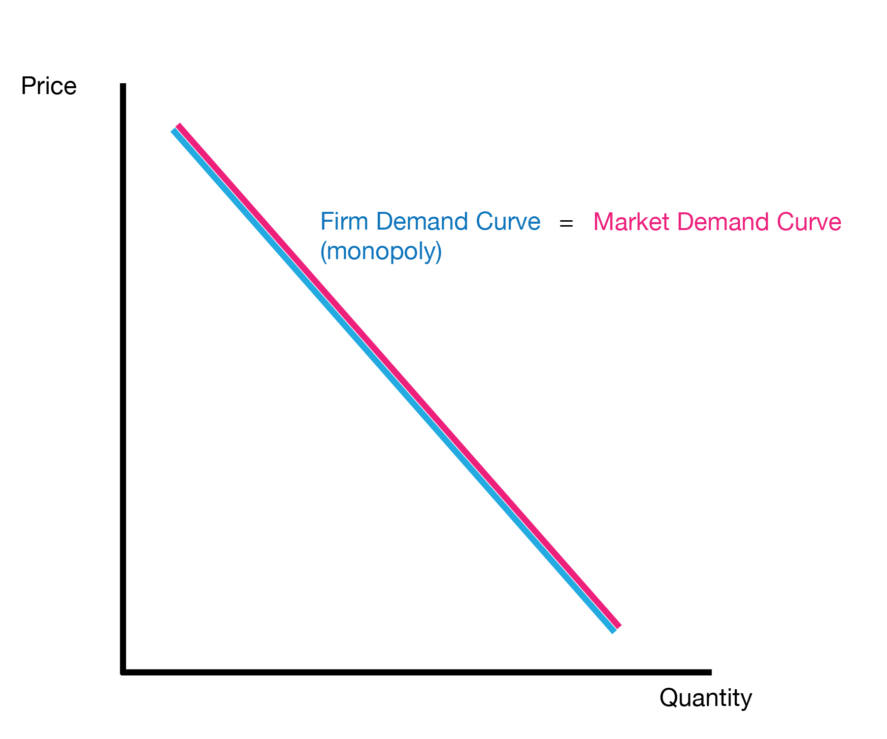
9.4 Monopoly
The extreme of market power is the monopoly, where there is only one seller in the market. For the monopolist, the firm demand curve is equal to the market demand curve. This occurs because the monopolist is the only firm in the market consumers can purchase from.
We now solve the monopolist’s problem. The monopolist wants to maximize their profit, which is equal to their revenue minus their total costs. We can view this under the benefit-cost framework, where the ‘benefit’ is revenue, and the ‘surplus’ is profit.
If we want to maximize total profit (surplus), we therefore choose the quantity where the marginal revenue (marginal benefit) equals the marginal cost.
The following table presents the monopolist’s problem in table form. Given the demand curve (represented by Price, Quantity pairs), the monopolist computes the marginal revenue and continues producing until it equals the marginal cost. In this example, the monopolist produces 3 units of the good.
What price does the monopolist charge? While the monopolist makes a profit, they are still bound by the demand curve. Once they’ve decided the quantity Q they want to charge, the monopolist uses the demand curve to find the price that sells that quantity. In this case, the monopolist sets the price to $22,000. Note this is not the same as the marginal revenue.
| Price (P) | Quantity (Q) | Total Revenue (P × Q) | Marginal Revenue | Marginal Cost | Profit |
|---|---|---|---|---|---|
| $24,000 | 1 | $24,000 | $24,000 | $20,000 | $4,000 |
| $23,000 | 2 | $46,000 | $22,000 | $20,000 | $6,000 |
| $22,000 | 3 | $66,000 | $20,000 | $20,000 | $6,000 |
| $21,000 | 4 | $84,000 | $18,000 | $20,000 | $4,000 |
| $20,000 | 5 | $100,000 | $16,000 | $20,000 | $0 |
We now present the problem in graph form. The monopolist finds the quantity on the x-axis where marginal revenue is equal to the marginal cost. They then look up to the demand curve to find the price that leads to that quantity demanded.
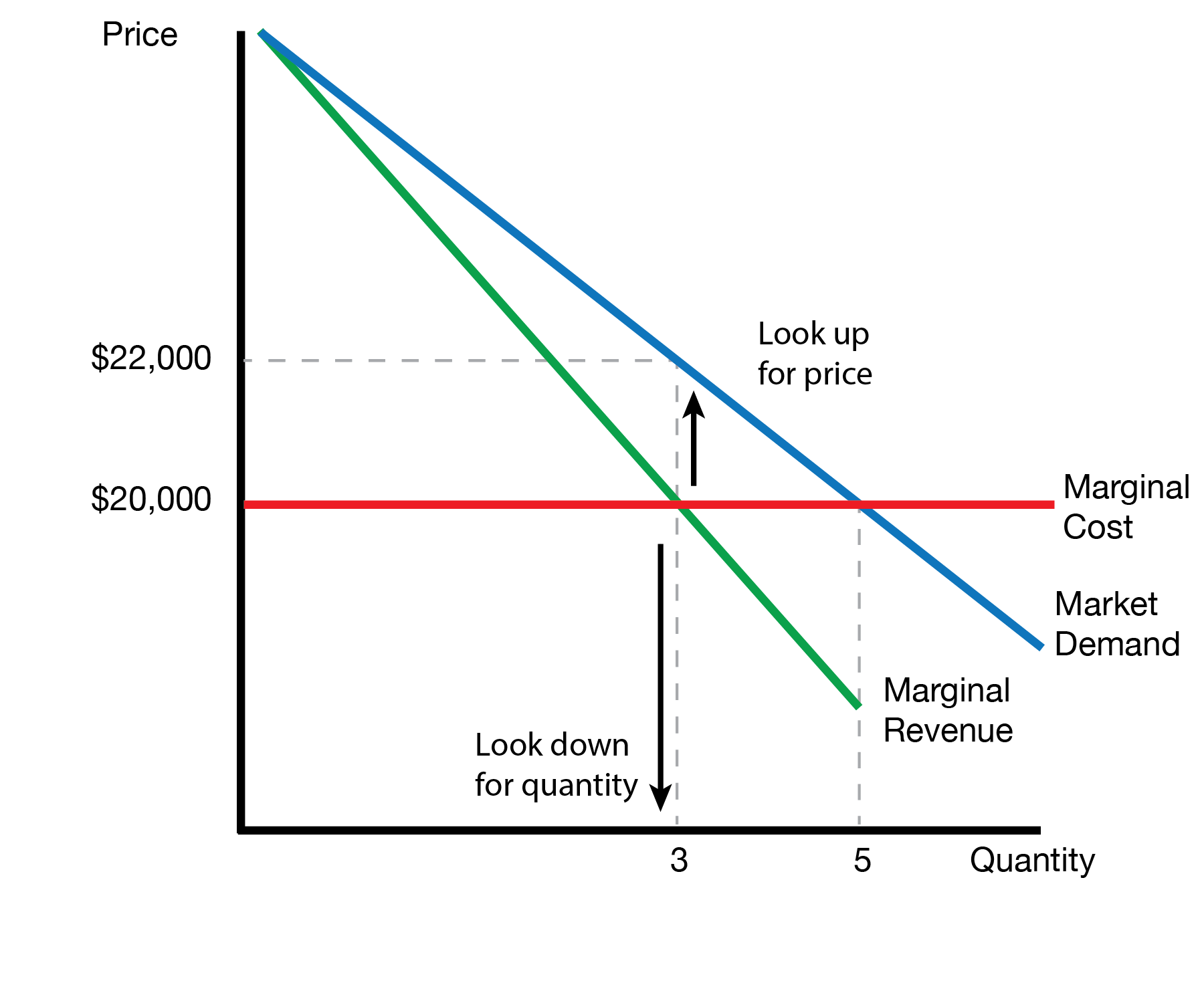
We now compare the monopolist’s choices with the competitive equilibrium. The monopolist chooses a higher price and lower quantity compared to the competitive equilibrium. The competivie equilibrium equates demand and supply. For a competitive market, supply is equal to the marginal cost curve. In this case, the equilibrium is given by the intersection where the price is $20,000 and the quantity is 5. This provides our competitive equilibrium.
| Monopolist | Competitive | |
|---|---|---|
| Quantity | Where Marginal Revenue = Marginal Cost | Where Demand = Marginal Cost |
| Price | Find quantity where Marginal Revenue = Marginal Cost Read price off demand curve |
Marginal Cost |
Notably, the monopolist underproduces and overcharges relative to the competitive equilirbium. We therefore view the monopolist as welfare reducing.
9.5 Conclusion
- This lecture introduces market power in which sellers have some power over the price they can set
- We introduce a spectrum of market power which ranges from perfect competition to full monopoly
- We solve the monopolist’s problem, which underproduces and overcharges relative to the social optimum