4 Equilibrium
Objectives
- Identify shortages and surpluses
- Identify a market equilibrium
4.1 Introduction
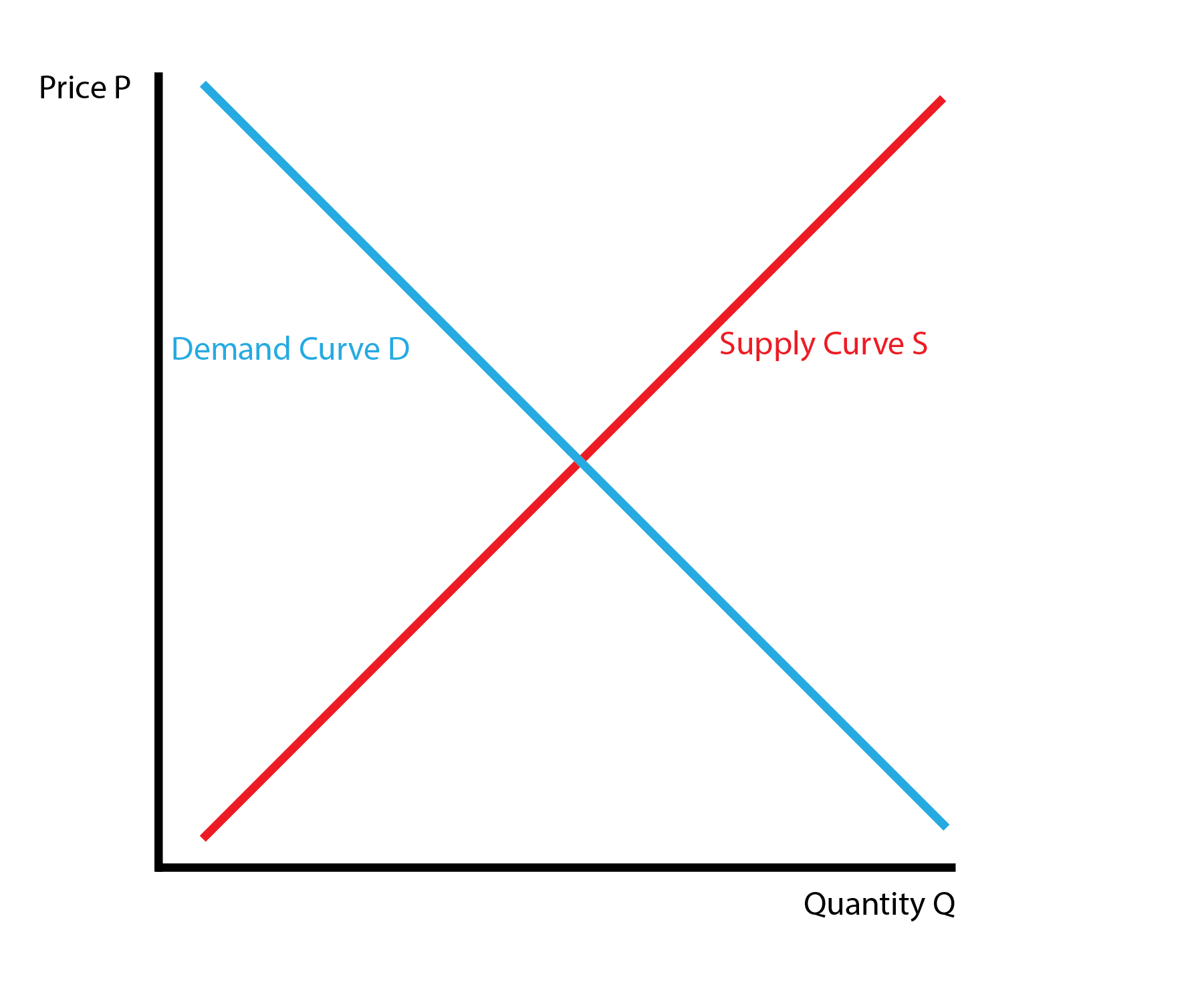
This lecture introduces the concept of equilibrium. The equilibrium is ‘where we end up’ in terms of the price and quantity of a good. Until now, we have the demand curve, which tells us how much consumers want to buy at each price, and the supply curve, which tells us how much producers want to sell at each price. The problem is we don’t know the actual price and quantity that will occur in the market yet, we only have a menu.
We will introduce the demand and supply curves together. Graphically, we simply draw them on the same graph:
4.2 Out of Equilibrium
We now consider different possible prices and quantites. We start by considering a price and then examining the quanties.
In the leftmost graph, we consider a low price. In this case, the quantity demanded exceeds the quantity supplied, which we call a shortage. How do we leave the shortage? Businesses know they can raise their price and still sell all their product, so the price will increase. Because the price has not settled, we are not in equilibrium.
In the rightmost graph, we consider a high price. In this case, the quantity supplied exceeds the quantity demanded, which we call a surplus. How do we leave the surplus? Businesses know they must lower their price to sell their excess product, so the price will decrease. Because the price has not settled, we are not in equilibrium.
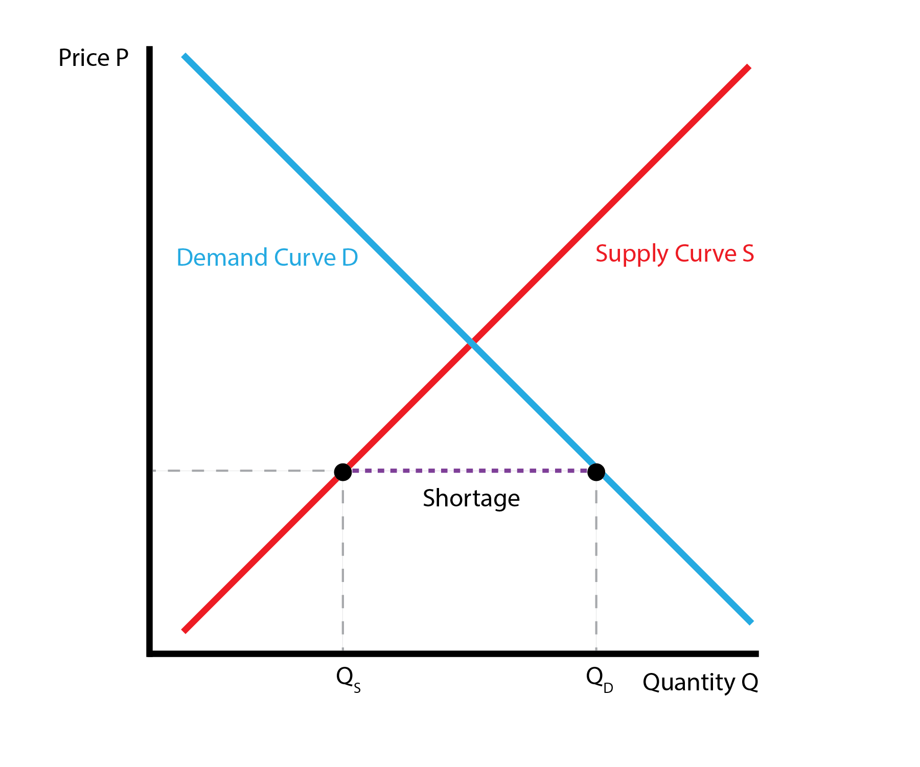
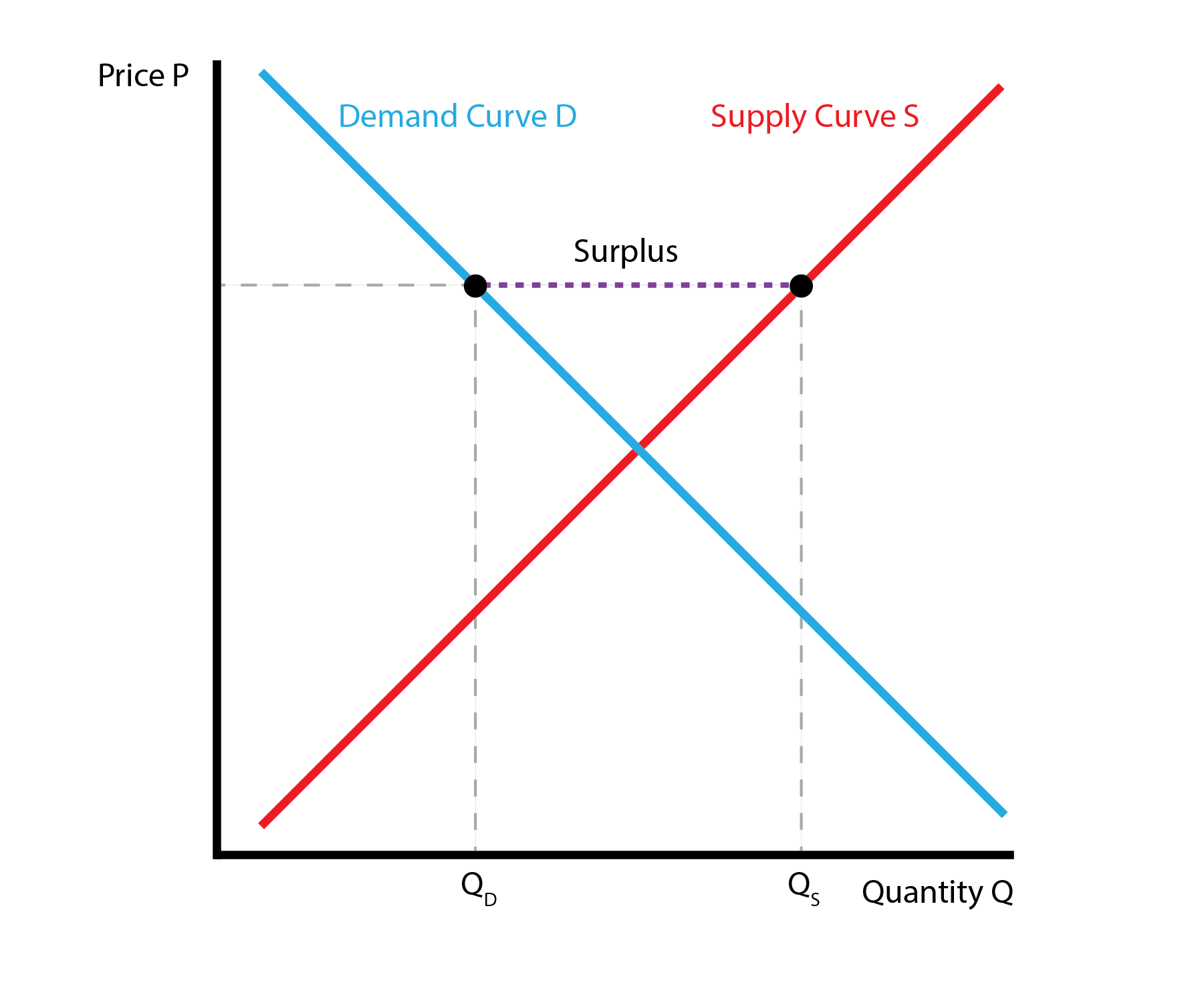
Out of Equilibrium: Shortage and Surplus
4.3 Equilibrium
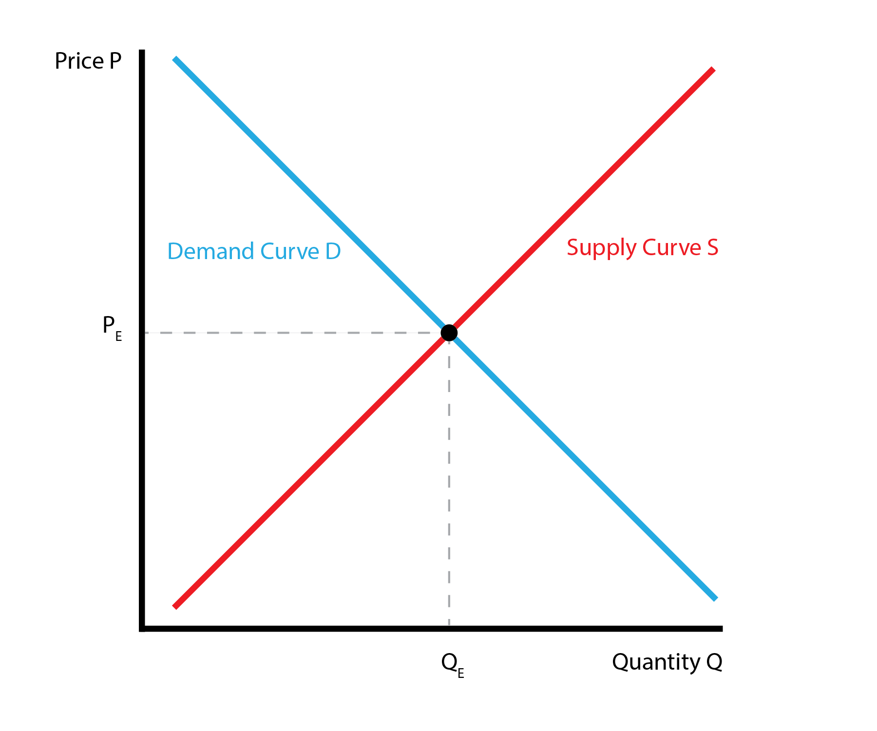
This leaves us one option: the price where quantity demanded equals quantity supplied. In this case we say the market has cleared: everybody that wants to buy good at that price can do so, and everybody that wants to sell the good at that price can do so. No has any incentive to either raise or lower the price, so the price has settled. This introduces a unique equilibrium quantity \(Q_E\) with associated equilibrium price \(P_E\).
4.4 Shifts
The demand and supply curves hold ‘everything else’ constant. But what happens when ‘everything else’ changes? When something else changes, the demand or supply curve will shift, leading to a new equilibrium price and quantity (If we look closely, the old equilibrium price will no longer clear the market). Demand and can supply can increase or decrease. This gives us \(2 \times 2 = 4\) possible shifts.
We first examine the demand shifts:
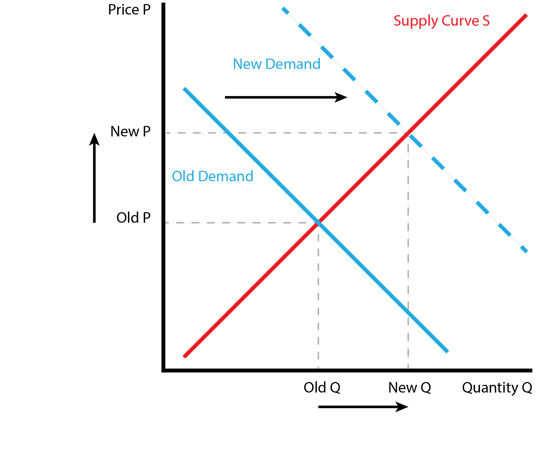
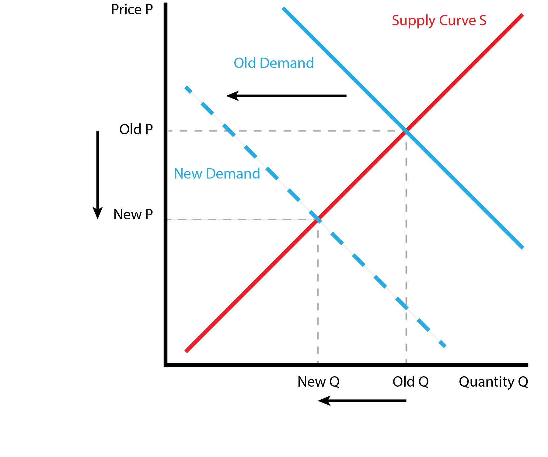
Demand Shifts
Now we examine the supply shifts:
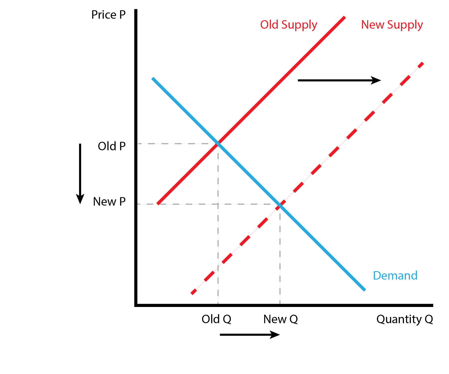
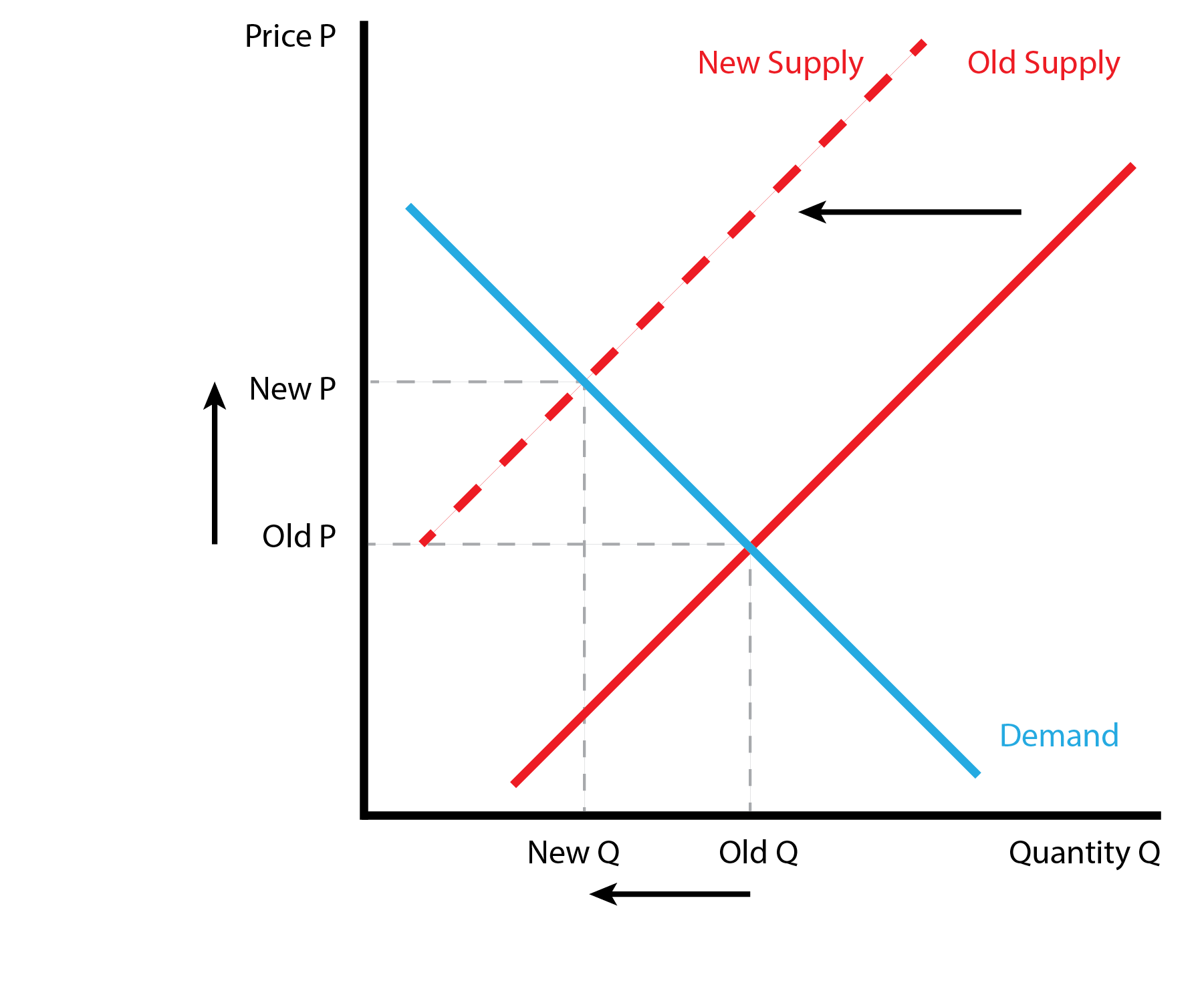
Supply Shifts
We can organize the results in the following table: Note that the demand and supply shifts have distinct signatures. Demand shifts leads price and quantity to move in the same direction, while supply shifts lead price and quantity to move in opposite directions.
| Shift | P (Price) | Q (Quantity) |
|---|---|---|
| Demand ↑ | ↑ Increase | ↑ Increase |
| Demand ↓ | ↓ Decrease | ↓ Decrease |
| Supply ↑ | ↓ Decrease | ↑ Increase |
| Supply ↓ | ↑ Increase | ↓ Decrease |
4.5 Conclusion
- This lecture combines the demand and supply curves to form the equilibrium
- The unique price and quantity with neither a surplus nor shortage
- We introduce our set of demand and supply shifts
- These shifts introduce changes in the equilibrium price and quantity