3 Supply
Objectives
- Know the definition of the supply curve
- Identify movements along the supply curve vs. shifts of the supply curve
- Know common shifts of the supply curve
- Input Prices
- Technology / Productivity
- Other Opportunities
- Expectations
- Types and number of sellers
- Know the relationship between the supply curve and the marginal cost curve
- Be able to compute the market supply curve
3.1 Introduction
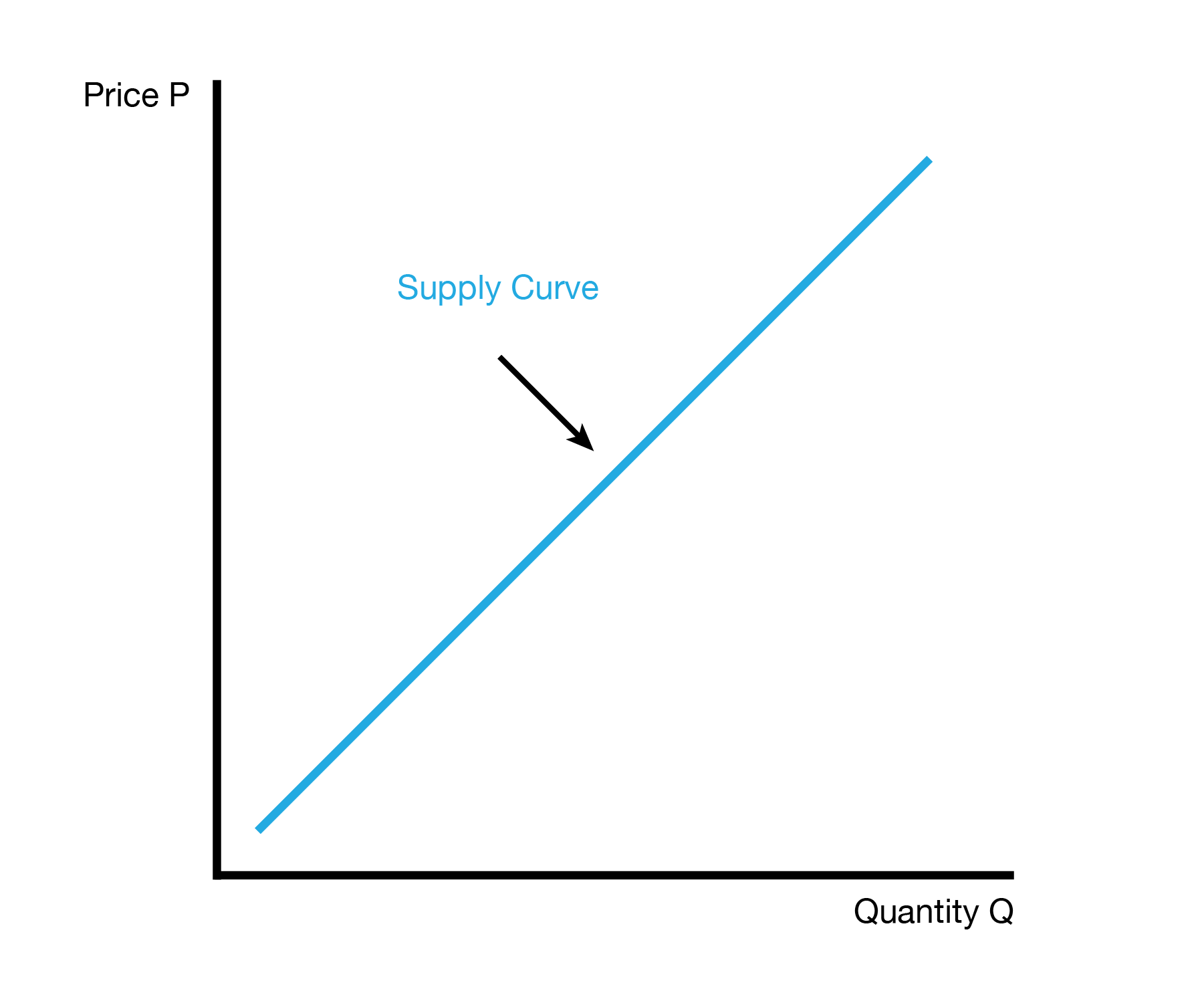
This section introduces the supply curve, which comes from the producer problem of how much of something we should produce. Our decision depends on many different factors: the price, the price of inputs, how productive we are, the competition. The supply curves isolates the relationship between the price and quantity supplied, holding everything else constant.
3.2 Movement Along the Supply Curve
We start by studying what happens when the price of a good changes. In this case we simply move along the supply curve. This includes two cases: a decrease in the price and an increase in the price.
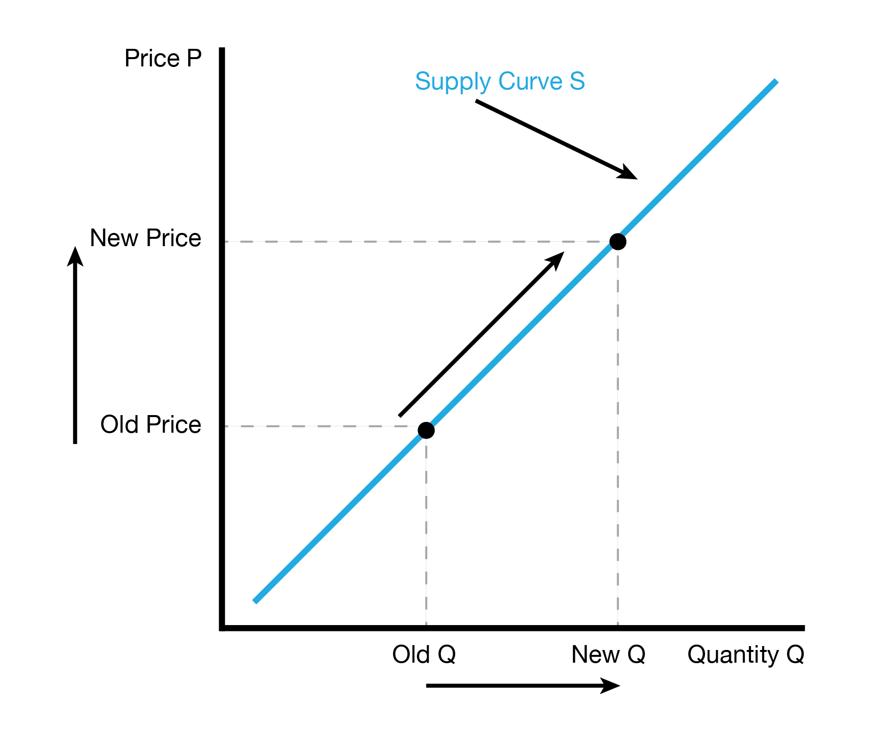
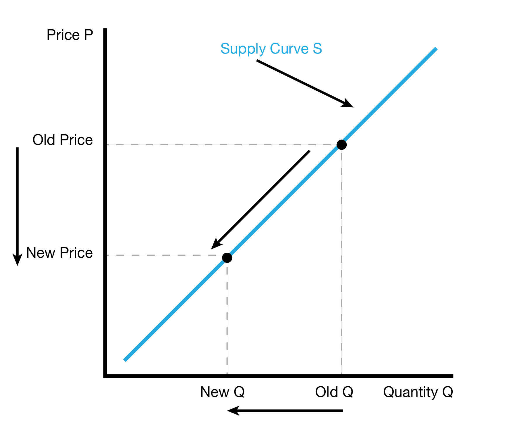
Movements Along the Supply Curve
3.3 Shifts of the Supply Curve
We now study what happens when ‘everything else’ changes. If we have a price change and want to study how our quantity supplied changes, we simply trace along the supply curve. When something else changes, we can no longer simply trace along the supply curve. In fact, the entire supply curve will shifts. This occurs because our quantity supplied changes at every price due to the outside factor.
There are two types of supply shifts: an increase in supply and a decrease in supply. When we have an increase in supply, we want to produce more of the good at every price. When we have a decrease in supply, we want to produce less of the good at every price. Note that on the graph, an increase in supply shifts the supply curve to the right, while a decrease in supply shifts the supply curve to the left. This differs from our usual intuition of a shift up or down.
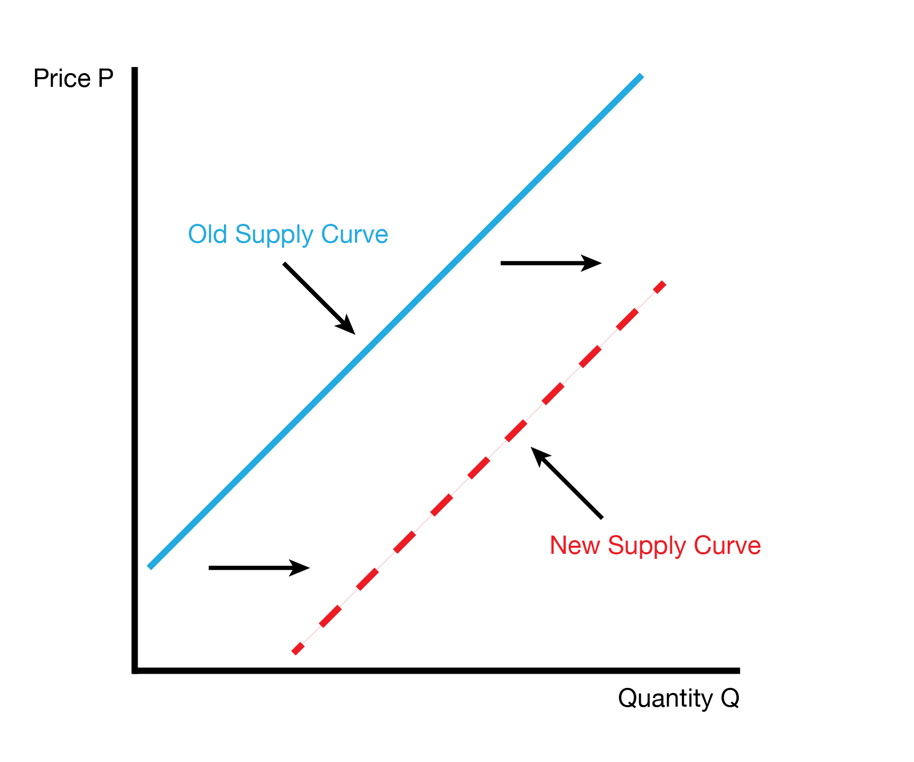
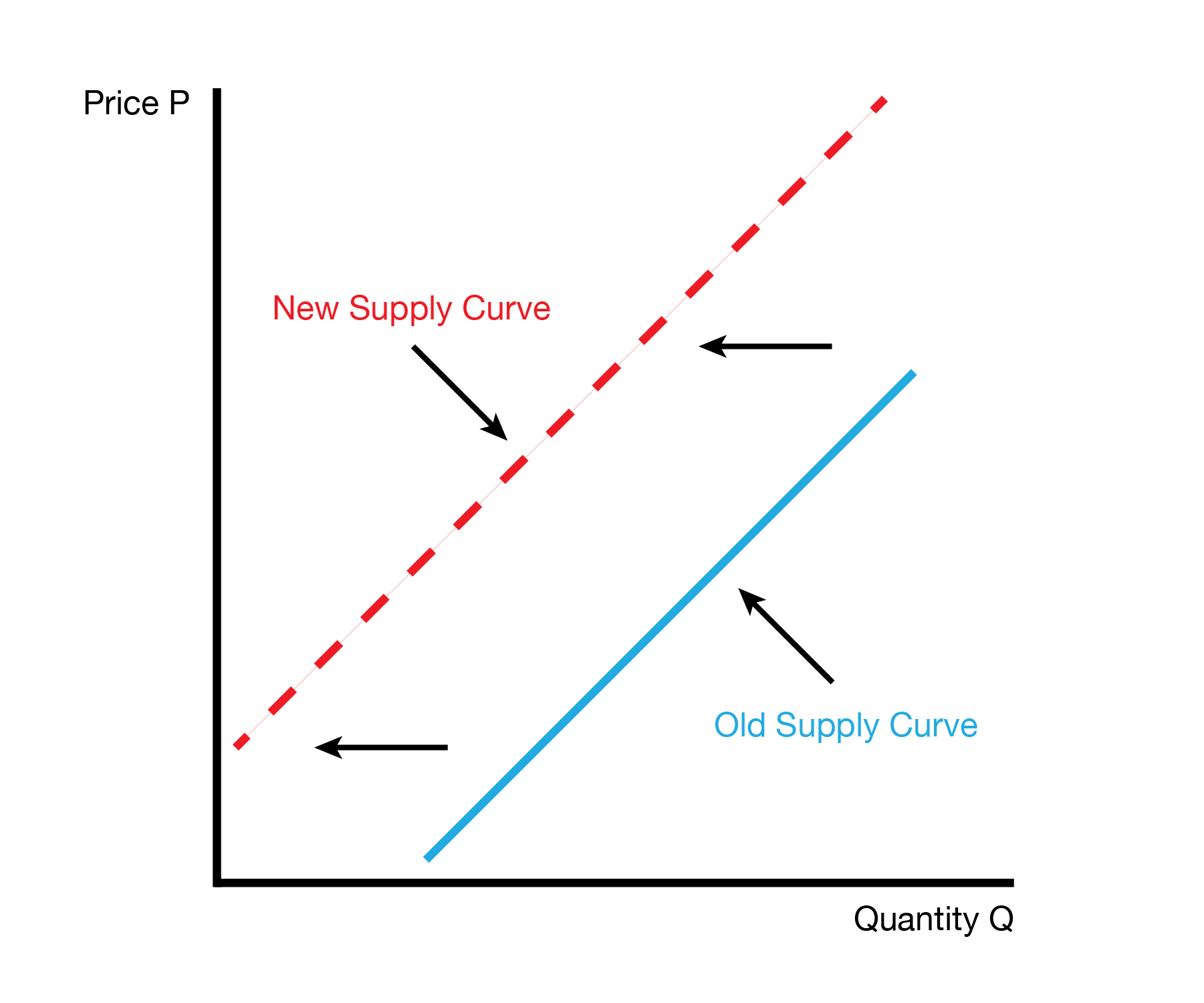
Supply Shifts
3.3.1 Input Prices
The majority of goods are made with other goods, which we call inputs. As the price of inputs increases, it becomes more expensive to produce the good. This makes it less profitable to produce the good, so we produce less of it at every price. As the price of inputs decreases, it becomes less expensive to produce the good. This makes it more profitable to produce the good, so we produce more of it at every price.
| Input Prices | Supply |
|---|---|
| Increase | Decrease |
| Decrease | Increase |
3.3.2 Technology / Productivity
Our catch all for how good we are at producing the good is called productivity or technology. When we become more productive, we can produce more of the good with the same amount of inputs. This makes it more profitable to produce the good, so we produce more of it at every price (supply increase). When we become less productive, we produce less of the good with the same amount of inputs. This makes it less profitable to produce the good, so we produce less of it at every price (supply decrease).
| Productivity and Technology | Supply |
|---|---|
| Increase | Increase |
| Decrease | Decrease |
3.3.3 Other Opportunities
Every business (producer) has opportunity to make other products. When the other opportunities become more attractive, we want to produce less of our current good at every price so that we can follow the more profitable opportunity (supply decrease). When the other opportunities become less attractive, we want to work on other opportunities less, so we can spend more time producing our current good (supply increase).
| Other Opportunities | Supply |
|---|---|
| More Attractive | Decrease |
| Less Attractive | Increase |
3.3.4 Prics in the Future: Expectations
Our supply of a good can depend on our expectations about the future. It’s important to distinguish between our supply today and our demand tomorrow. Our generic supply curve refers to our demand today as a function of today’s price. When the price in the future changes, it can affect our supply today as an outside factor.
If we expect a higher price in the future, we want to hold back some of our supply today to sell more in the future at the higher price. This leads to a decrease in our supply today. If we expect a lower price in the future, we want to sell more of our supply today before the price drops. This leads to an increase in our supply today.
| Price in the future | (Today’s) Supply |
|---|---|
| Increase | Decrease |
| Decrease | Increase |
3.4 The Supply Curve and the Marginal Cost Curve
One of the most important results in economics is that the demand curve is equal to the marginal benefit curve. The reason why is as follows: - Each point on the supply curve tells us the lowest price a producer is willing to accept for that extra unit. - That “minimum acceptable price” is exactly the marginal cost—because it’s the amount needed to cover the cost of producing one more unit.
So, the supply curve is just a graph of marginal cost: higher prices make it worthwhile to produce more, while lower prices limit production to units with lower marginal costs.
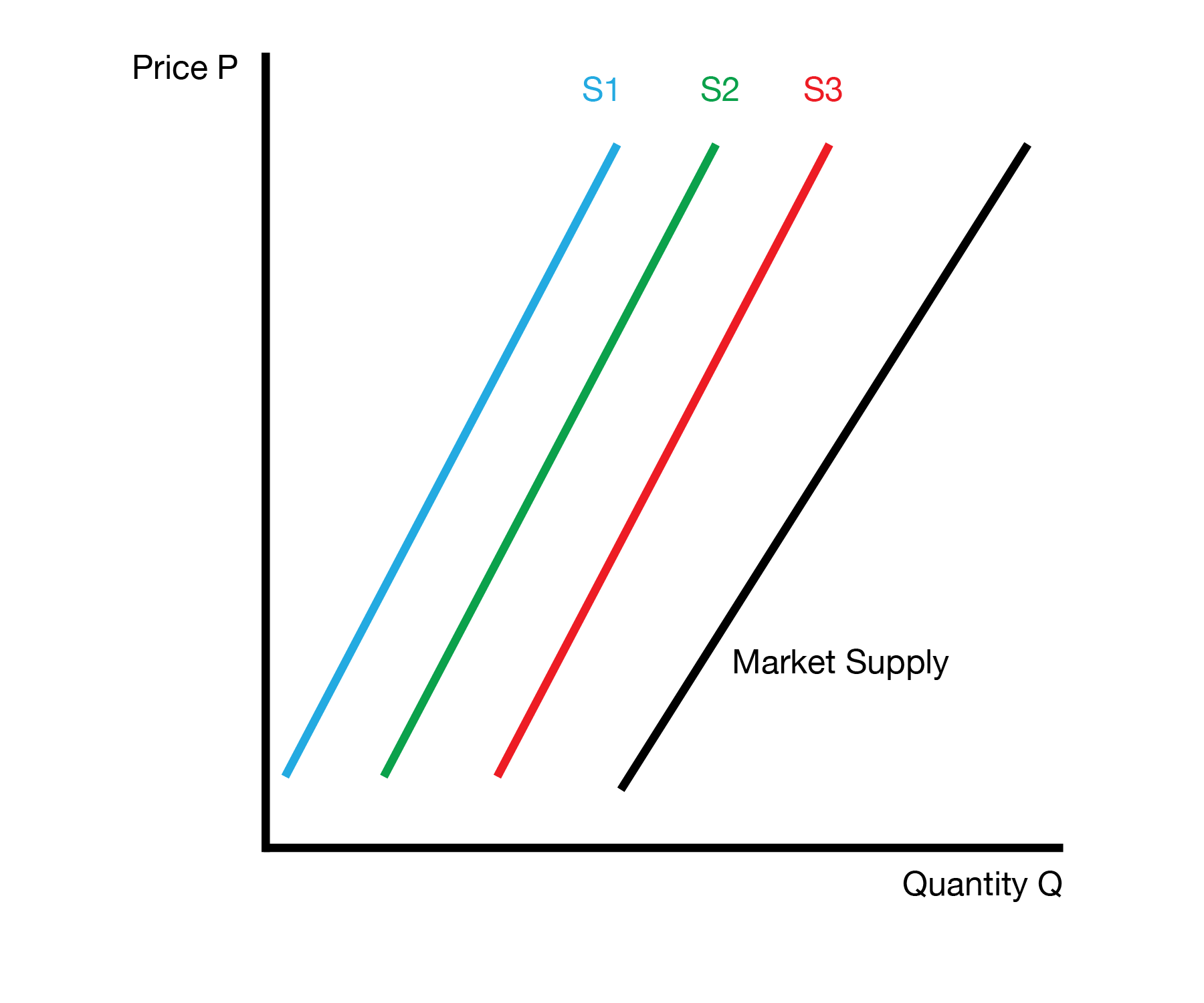
3.5 Market Supply
If we’re competing against other firms, we might want to know the total supply for our product, not just our supply. We compute the market supply by simply adding the supply curves of all the individual consumers in the market. The only catch is that we need to add the quantities supplied at each price, e.g. we need to add horizontally, not vertically.
We can see this in the following example:
| P | S-McDonald’s | S-Wendy’s | S-Taco Bell | S-Market |
|---|---|---|---|---|
| 20 | 5 | 8 | 3 | 16 |
| 15 | 4 | 7 | 2 | 13 |
| 10 | 3 | 5 | 1 | 9 |
| 5 | 2 | 2 | 0 | 4 |
| 0 | 0 | 0 | 0 | 0 |
Graphically, we can interpret the market supply curve as the horizontal sum of each individual supply curve.
3.6 Conclusion
- This lecture studies the supply curve of the producer problem
- The supply curve isolates the relationship between the price and quantity supplied
- Changes in things other than the price (everything else) lead to supply shifts
- We show the supply curve is equal to the marginal cost curve and how to compute the market supply curve