4 Heckscher-Ohlin Model
Objectives
- Build trade equilibrium in the Heckscher-Ohlin model
- Understand the Stolper-Samuelson theorem
- Be able to identify winners and losers based on factor abundance
This lecture will develop the Heckscher-Ohlin model of trade. The Heckscher-Ohline model only features two factors of production: capital and labor.
We will assume Home has a stock of labor \(\overline{L}\) and a stock of capital \(\overline{K}\). Each factor can be used in the production of two goods: computers (C) and shoes (S). We will assume both goods are produced using both factors of production, and the factors can move freely across industries. Because we allow for free movement, we view the Heckscher-Ohlin model as capturing the long run rather than the short run. The idea is that in the short run, capital and labor can’t refactor into different industries: machines are built for a specific industry and workers are trained for a specific industry. In the long run, we build new machines and train new workers, so they can move freely across industries.
We represent this as the following equations: \[ \begin{aligned} \overline{L} &= L_C + L_S \\ \overline{K} &= K_C + K_S. \end{aligned} \]
The total stock of labor is used in the computer industry (\(L_C\)) and the shoe industry (\(L_S\)), and similarly for capital. This captures free movement because any combination of \(L_C\) and \(L_S\) works as long as we respect the grand total.
We will assume shoes are labor intensive and computers are capital intensive. The labor intensity of shoes is given by the assumption \[ \frac{L_S}{K_S} > \frac{L_C}{K_C}, \] that is shoes use relatively more labor than computers (this is only about the ratio or ‘recipe’. We don’t know the total amounts of labor and capital used in each industry).
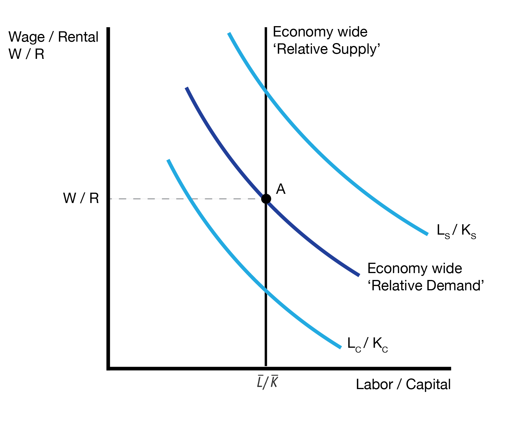
We express this graphically using the relative demand graph:
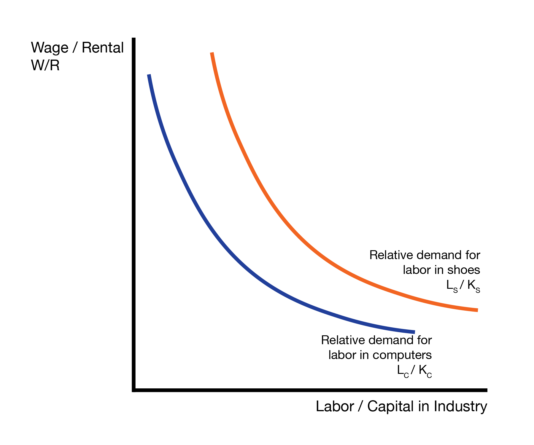
For a given ‘relative price of labor’ \(W/R\), the shoe industry demand ‘relatively’ more labor than the computer industry, \(L_S/K_S > L_C/K_C\).
We also need to consider foreign, who has their own labor and capital stocks \(\overline{L}^*\) and \(\overline{K}^*\). We will assume Home is capital abundant and Foreign is labor abundant: \[ \frac{\overline{K}}{\overline{L}} > \frac{\overline{K}^*}{\overline{L}^*}. \] This means home has ‘relatively’ more capital than foreign.
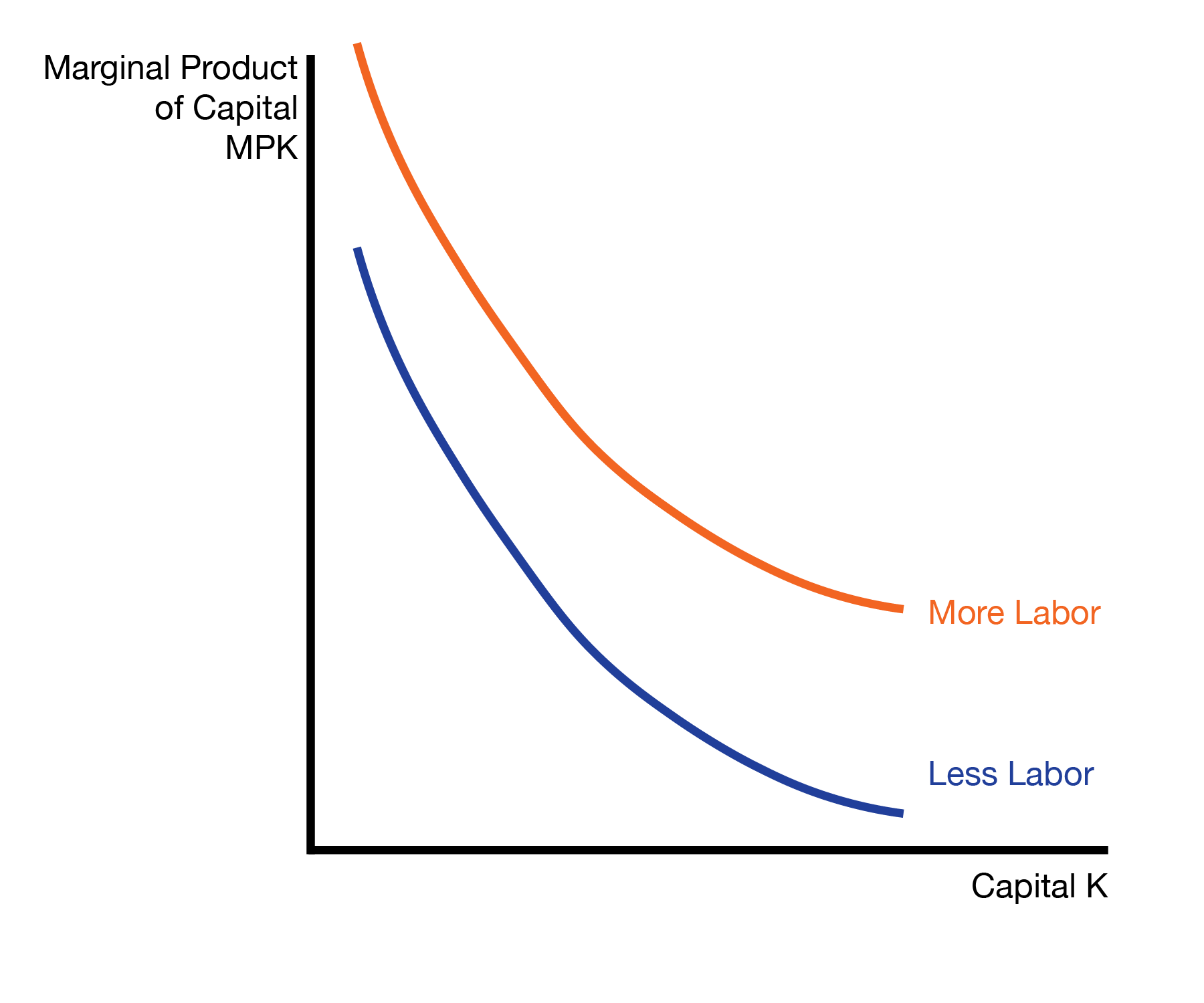
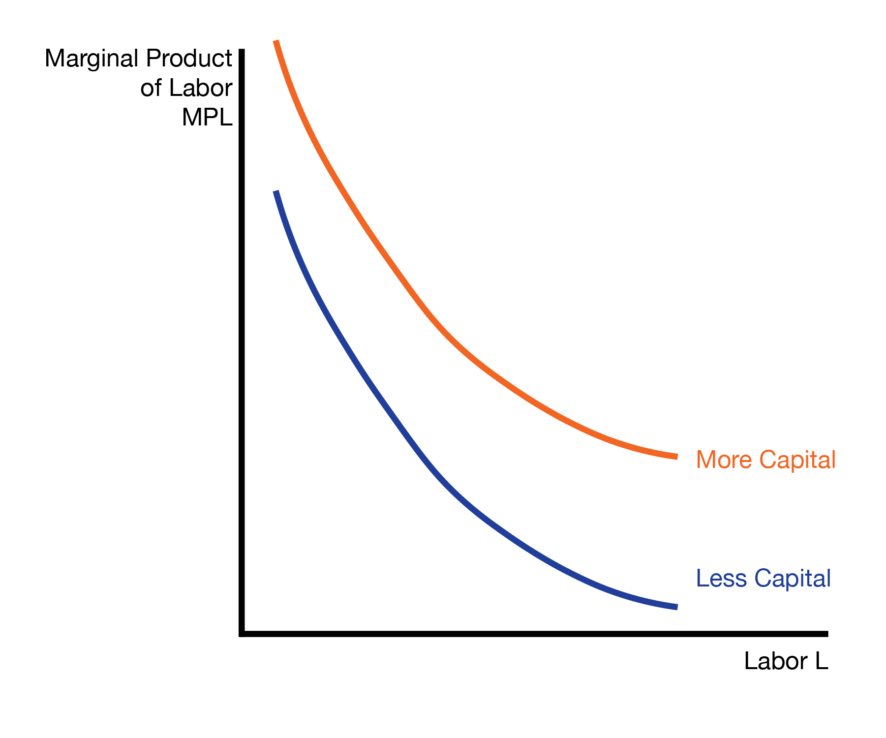
We will assume that the marginal productivity of capital (MPK) is increasing in labor and the marginal productivity of labor (MPL) is increasing in capital. The intuition is that with more labor workers, each unit of capital (each machine) is more productive. Equivalently, with more capital (machines or tools), each worker is more productive.
Finally, capital is paid the rental rate \(R\), and labor is paid the wage \(W\).
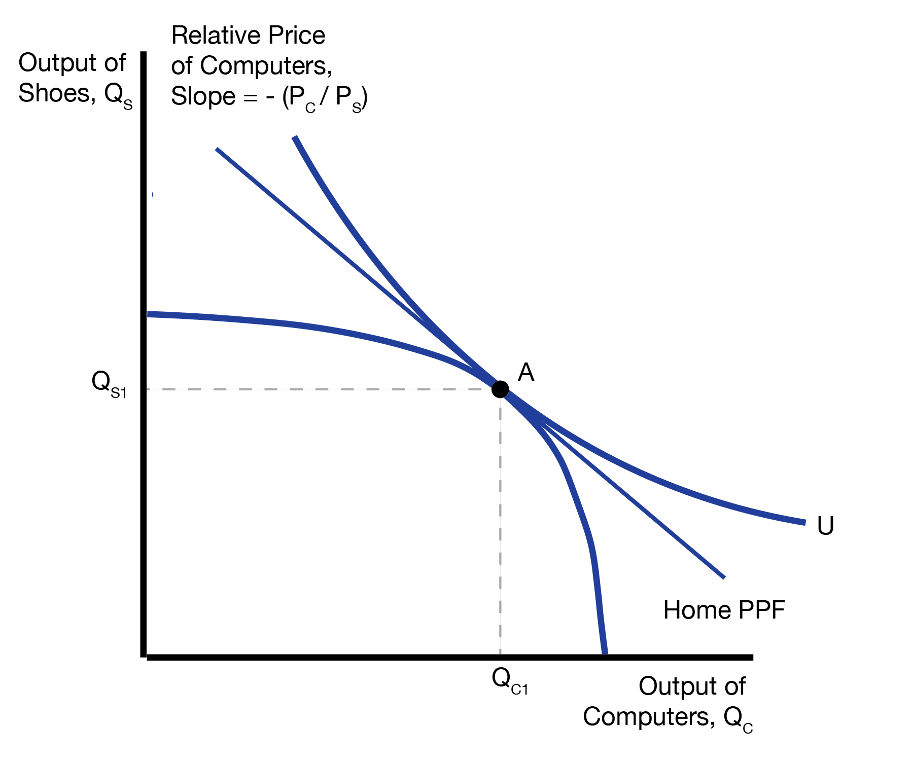
4.1 Autarky Equilibrium
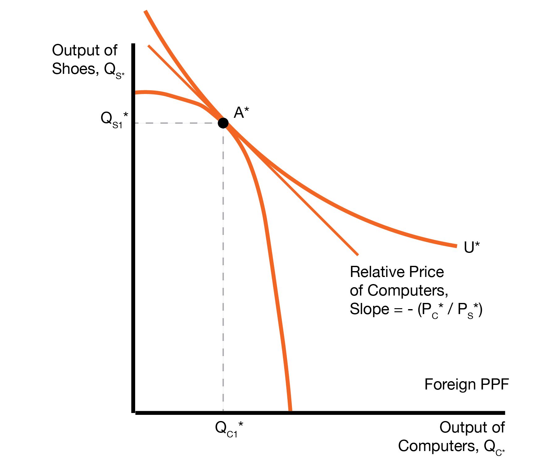
The autarky equilibria for Home and Foreign are given below. We will assume the autarky relative price of computers in Home is lower than in Foreign, \((P_C/P_S)^A < (P_C^*/P_S^*)^A\). The intuition is that Home is capital abundant, and computers are capital intensive, so it is easy for Home to produce computers. Because it’s easy to make computers, they are cheap in Home relative to Foreign.
4.2 Trade Equilibrium
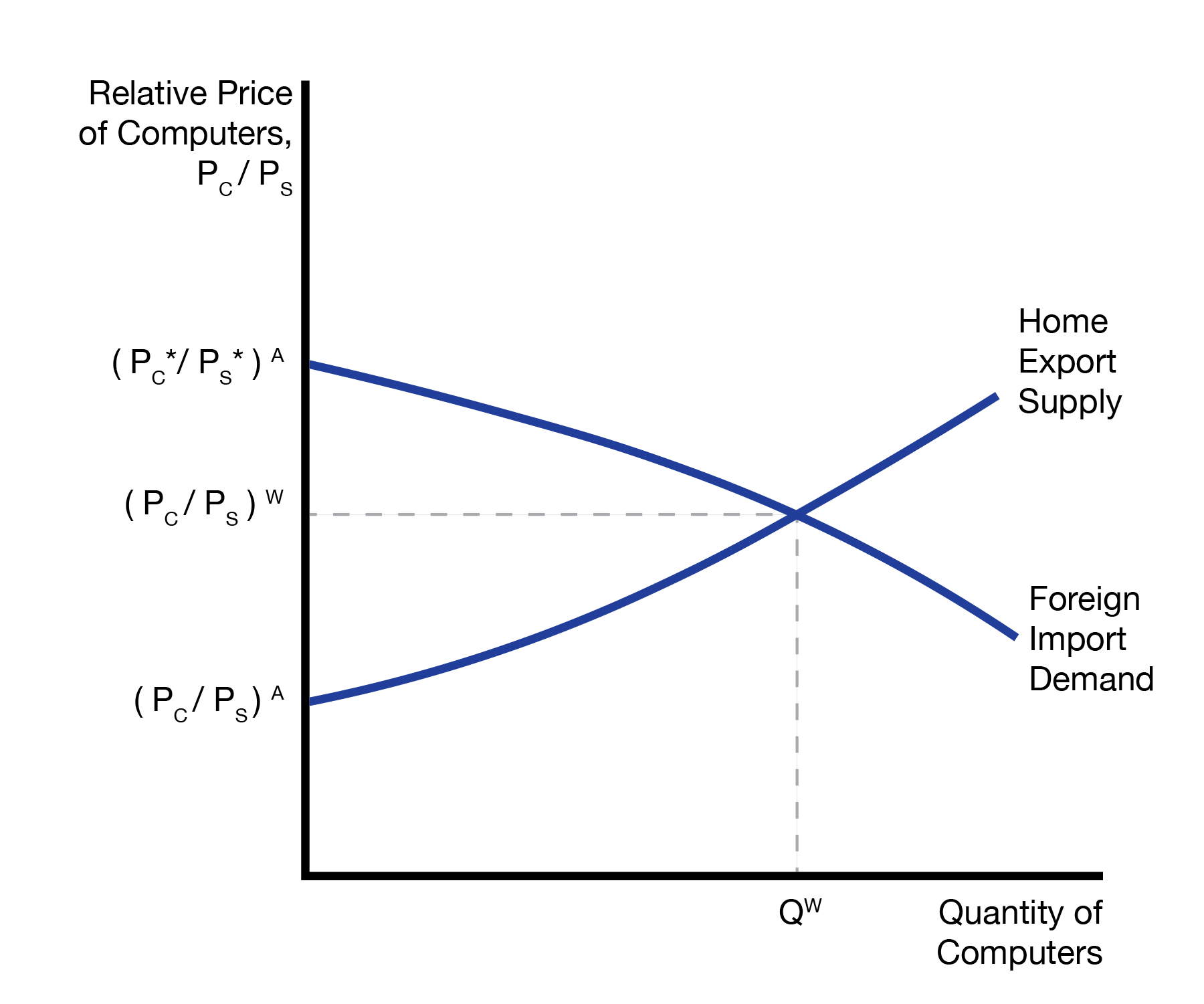
We will assume an increasing export supply curve of computers from Home, and decreasing import demand curve for computers from Foreign, drawn below. This provides the equilibrium trade price \((P_C / P_S)^W\) which is above the autarky price \((P_C / P_S)^A\).
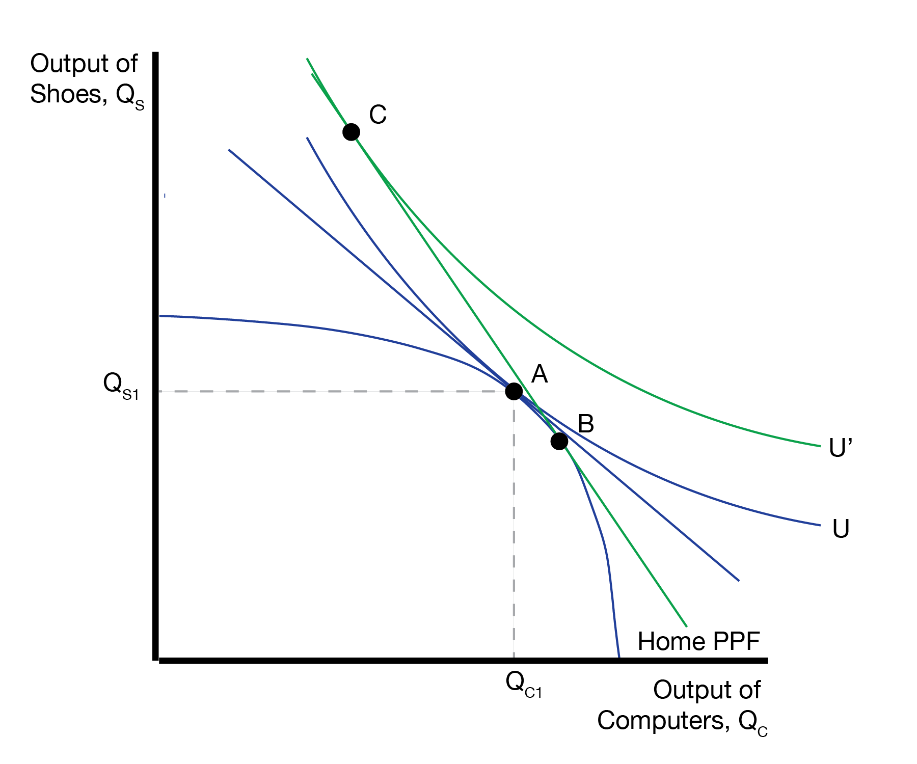
Given the new trade price, Home and Foreign now have to make the same choices they had to make once trade was introduced in the Ricardian and Specific Factors models. First, they decide where to produce, denoted by point \(B\) on the PPF. Second, they decide where to consume, denoted by point \(C\) on the trading curve.
The optimal production point is where the PPF is tangent to the trading curve, which has slope given by the relative price of computers to shoes \((P_C / P_S)^W\). Given this production point, households trade along the trading curve to their optimal consumption point \(C\), which is also tangent to the trading curve. Because the new indifference curve is higher than the autarky indifference curve, households are better off with trade. In this case, Home will export computers and import shoes.
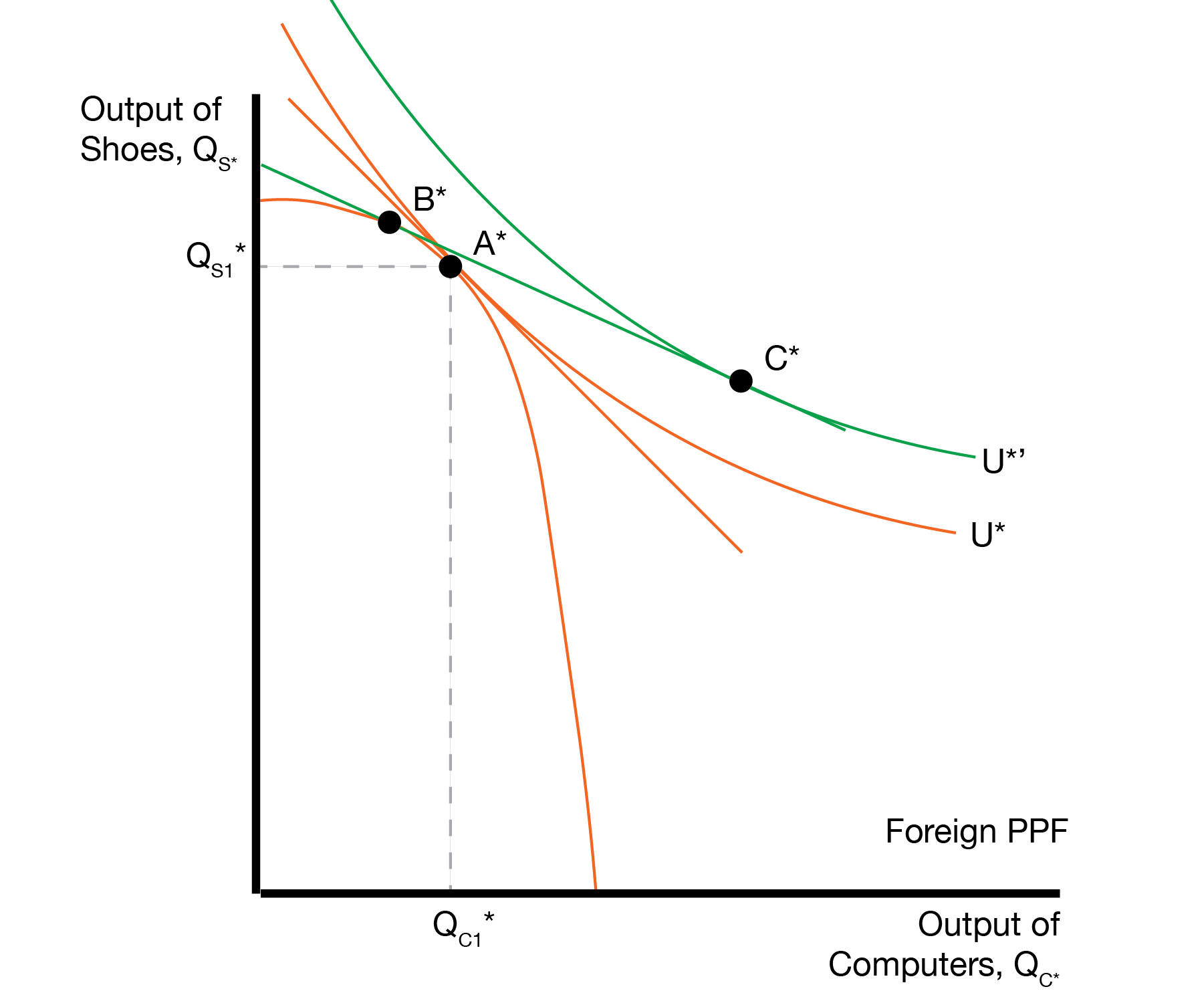
Foreign makes similar choices, producing at point \(B^*\) and consuming at point \(C^*\).
4.3 Winners and Losers
We now visit our two factors of production to see who wins and who possibly loses from trade.
Recall that capital earns rental rate \(R\). Each industry hires capital until the cost of capital \(R\) equals the marginal revenue product of capital. This provides two equations: \[ \begin{aligned} R &= P_C \times MPK_C \\ R &= P_S \times MPK_S. \end{aligned} \] We can then compute how many computers and shoes capital can purchase as \[ \begin{aligned} \text{Number of computers} = R / P_C &= MPK_C \\ \text{Number of shoes} = R / P_S &= MPK_S \end{aligned} \] It’s therefore enough to know how \(MPK_C\) and \(MPK_S\) change.
Similarly, labor earns wage \(W\). We can solve for the number of computers and shoes labor can purchase as \[ \begin{aligned} \text{Number of computers} = W / P_C &= MPL_C \\ \text{Number of shoes} = W / P_S &= MPL_S. \end{aligned} \]
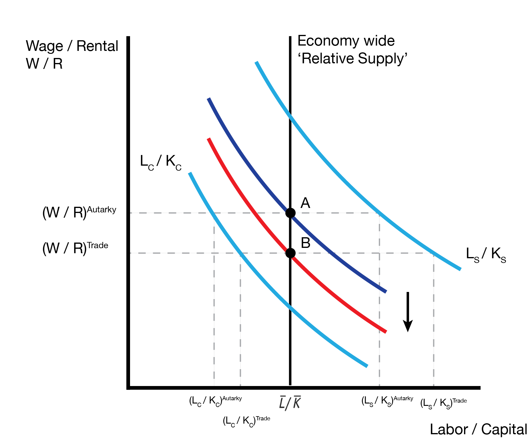
We will start by decomposing the total ‘relative’ labor supply as \[ \frac{\bar{L}}{\bar{K}} = \frac{\bar{L}_C + \bar{L}_S}{\bar{K}} = \frac{L_C}{K_C} \times \frac{K_C}{\bar{K}} + \frac{L_S}{K_S} \times \frac{K_S}{\bar{K}} \]
After trade we start producing more computers and less shoes, so \(K_C\) has increased and \(K_S\) has decreased. We can interpret this as a downward shift in the relative demand curve of the economy. Further, we can see the labor to capital ratio has increased in each indudstry.
We therefore have an increase in the marginal productivity of capital in computers \(MPK_C\) and shoes \(MPK_S\). This implies that capital owners are better off after trade. In contrast, we have a decrease in the marginal productivity of labor in computers \(MPL_C\) and shoes \(MPL_S\). This implies that labor is worse off after trade.
We summarize the effects of trade on the two factors of production in the following table.
| P of Capital Intensive Good Increases | P of Labor Intensive Good Increases | |
|---|---|---|
| Capital | Better off | Worse off |
| Labor | Worse off | Better off |
This result is called the Stolper-Samuelson theorem. When all factors are mobile, an increase in the relative price of a good will increase the real earnings of the factor used intensively in the production of that good and decrease the real earnings of the other factor.
4.4 Conclusion
- We’ve developed our trade equilibrium for the Heckscher-Ohlin Model
- The most important finding is the Stolper-Samuelson Theorem
- An increase in the relative price of a good will increase the real earnings of the factor used intensively in that good
- E.g. the factor that benefits is that used intensively in the exporting sector
- The Heckscher-Ohlin Model has a different motivation for trade
- Different countries have different endowments of capital and labor