3 Specific Factors Model
Objectives
- Build and identify a Specific Factors ‘trade equilibrium’
- Identify gains from trade in the trade equilibrium
- Identify winners and losers from trade
- Be able to identify trade flows based on relative prices and comparative advantage
3.1 Introduction
This lecture develops the specific factors model.
The specific factors model is a short-run model of trade that assumes that some factors of production are specific to an industry. We will assume there are two goods, manufacturing and agriculture, and three factors of production: labor, capital, and land. Labor is mobile between industries, but capital is specific to manufacturing and land is specific to agriculture.
The challenge of the Ricardian model is that there is only one factor of production, labor. If that factor loses from trade, it will revert to autarky. Therefore, we cannot have a ‘loser’ from trade in the Ricardian model. By allowing for multiple and specific factors of production, we want to see if the specific factors model can have a ‘loser’ from trade.
3.2 Assumptions
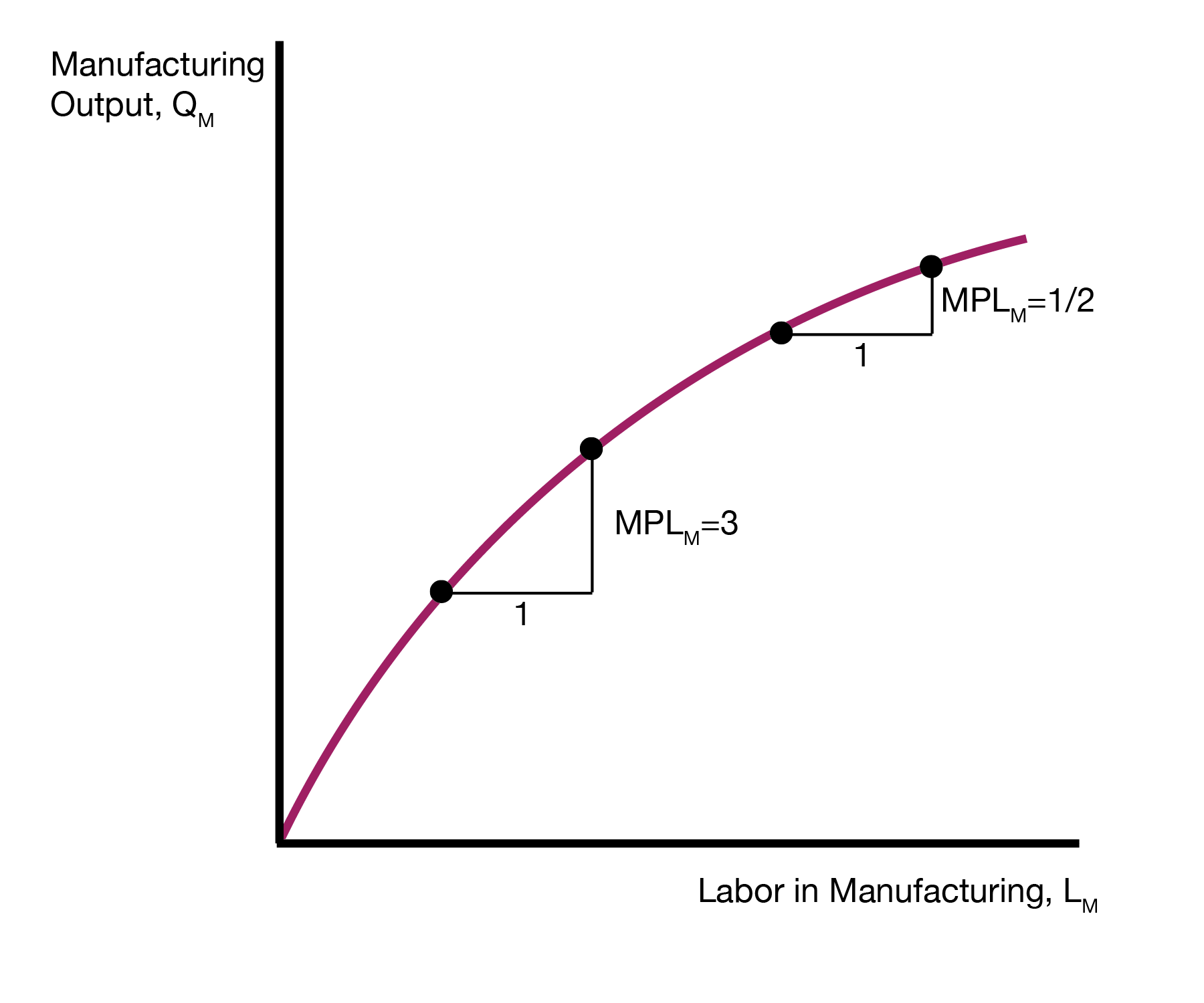
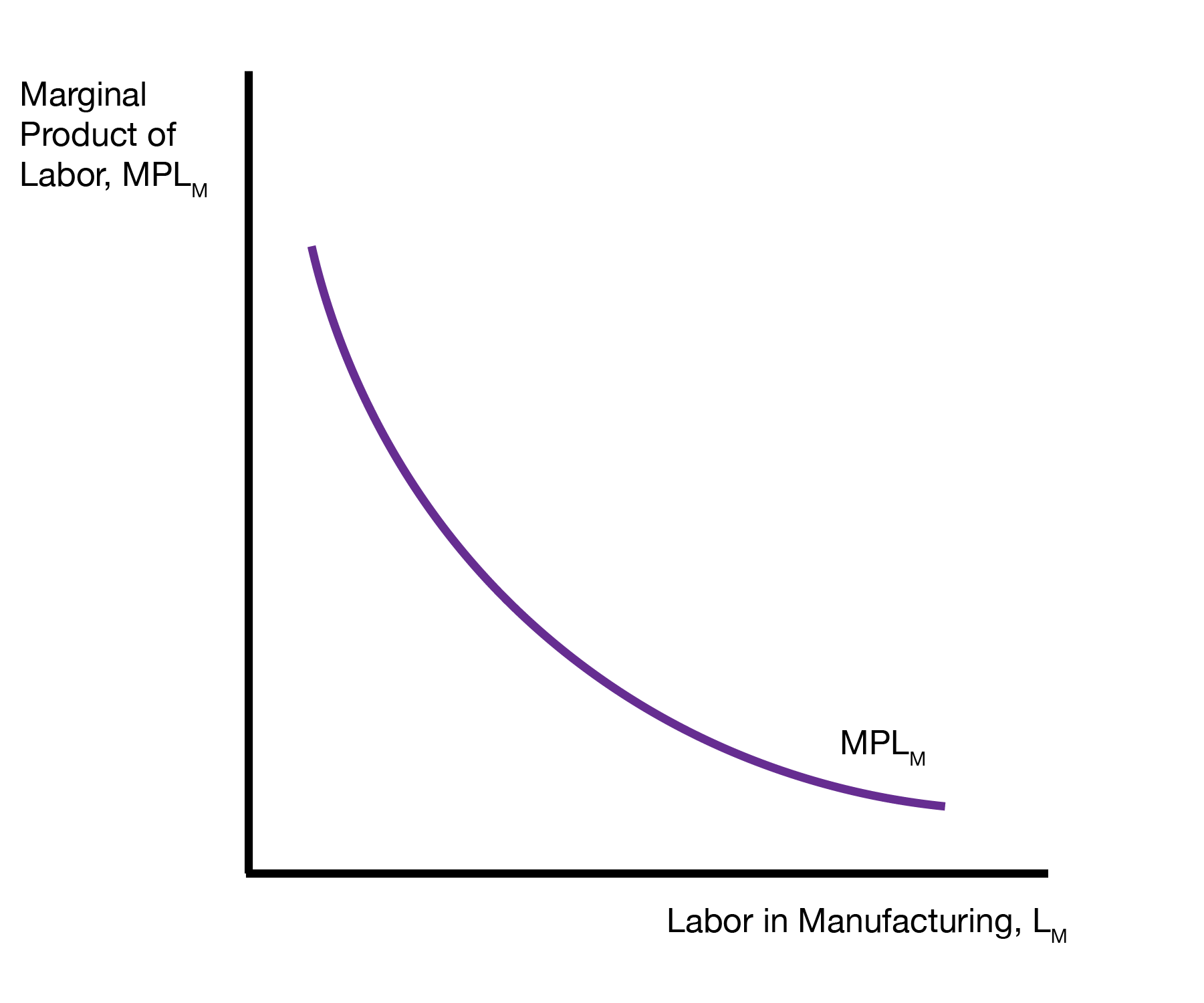
We will assume that manufacturing and agriculture both feature diminishing returns of labor usage. Diminishing returns states that as we use more labor in an industry, the marginal product (additional output from each unit of labor) of labor declines. This results in an increasing but concave output function.
3.3 Autarky Equilibrium
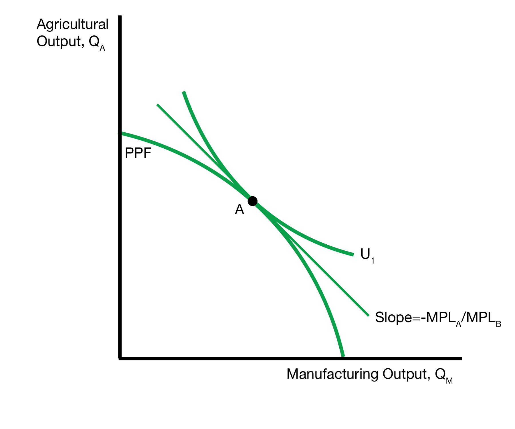
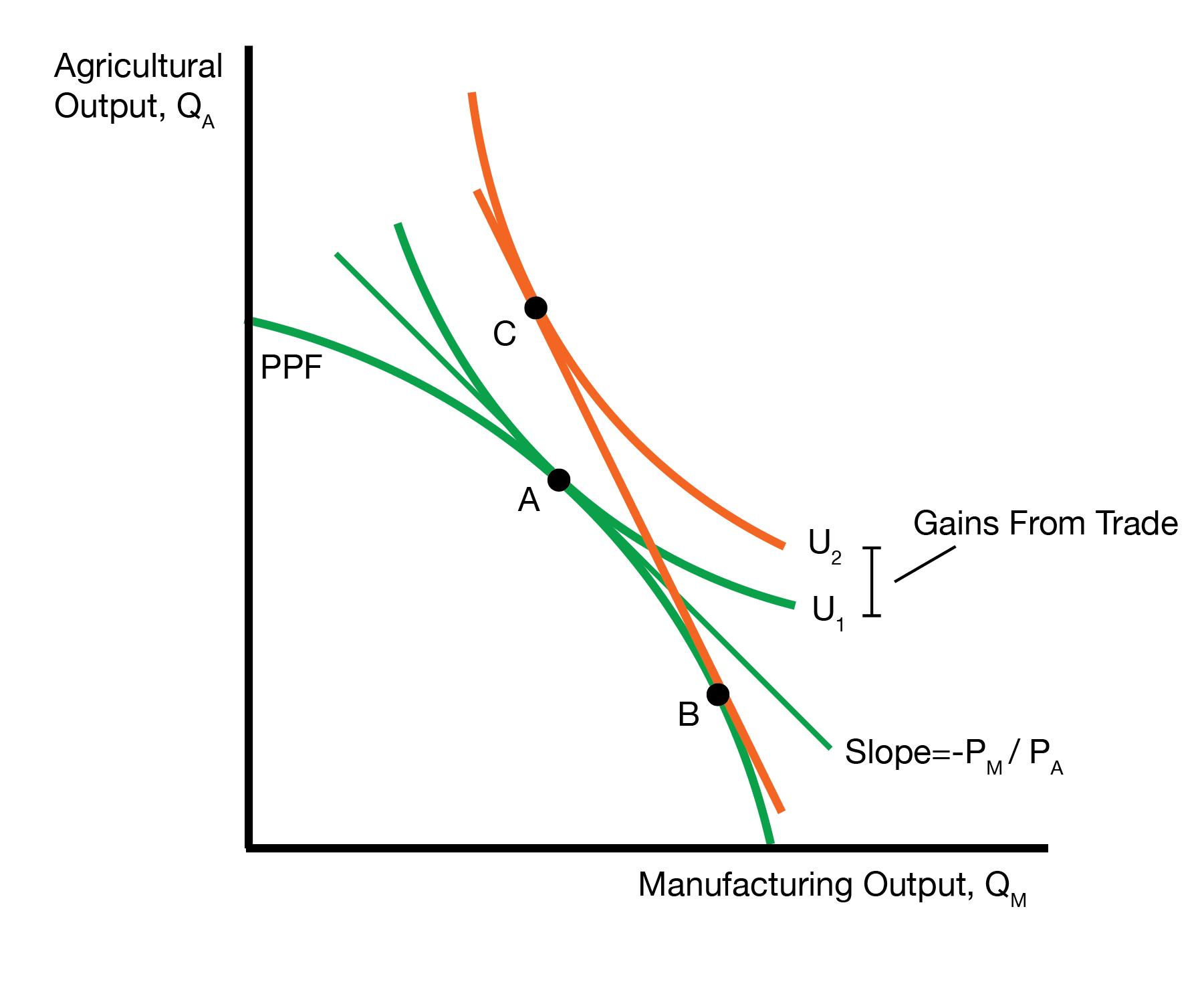
We first visit the autarky equilibrium, which serves as our baseline. The autarky equilibrium includes two markets: the goods market for manufacturing and agriculture, and the labor market. The leftmost figure displays the autarky equilibrium in the goods market. The production possibilities frontier (PPF) details possible production choices. Indifference curves represent consumer preferences. The consumption point A is where the highest indifference curve is tangent to the PPF.
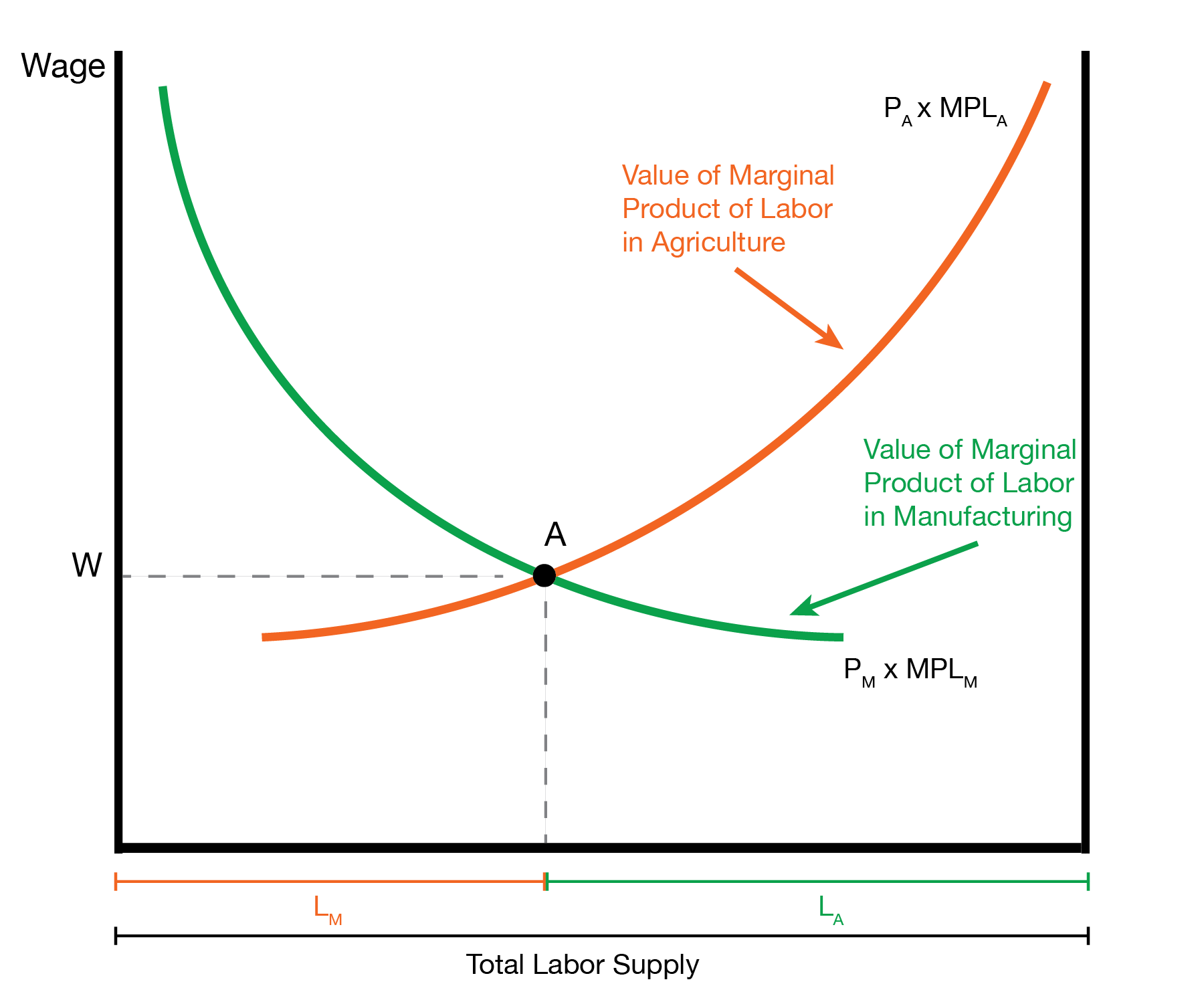
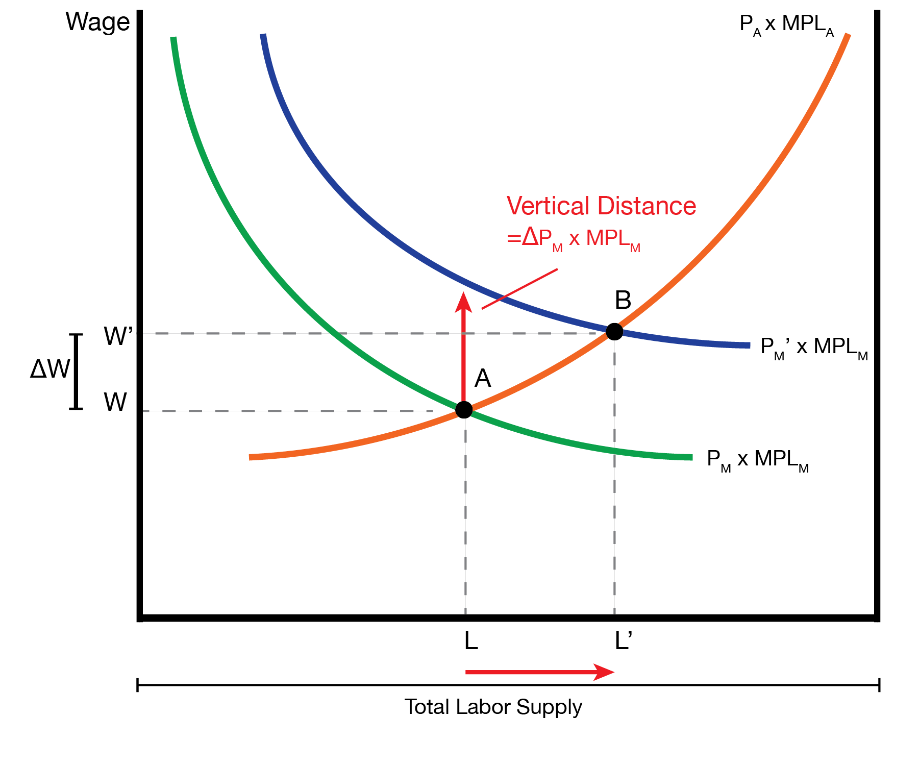
The rightmost figures displays the autarky equilibrium in the labor market. This figures is unique in that it includes the labor market for both manufacturing and agriculture. The assumption is that we have a fixed amount of labor \(L\) which can always be split as \(\overline{L} = L_M + L_A\). The leftmost green curve displays the marginal revenue product of labor in manufacturing, \(P_M \times MPL_M (L_M)\). But if there \(L_M\) units of labor in manufacturing, then there are \(L_A = \overline{L} - L_M\) units of labor in agriculture. This allows us to plot the marginal revenue product of labor in agriculture, \(P_A \times MPL_A (L_A)\).
We will assume the firm hire labor until the marginal revenue product of labor equals the wage. In manufacturing, this provides \(W_M = P_M \times MPL_M\). In agriculture, this provides \(W_A = P_A \times MPL_A\).
We now consider it from the workers’ perspective. If manufacturing pays a higher wage than agriculture, \(W_M > W_A\) then workers will move to manufacturing and abandon agriculture. If agriculture pays a higher wage than manufacturing, \(W_A > W_M\), then workers will move to agriculture and abandon manufacturing. Therefore, if we have workers in both industries, we must have \(W_M = W_A\). But this means \(P_M \times MPL_M (L_M) = P_A \times MPL_A (L_A)\). Graphically, we interpret this as the point where the two curves intersect.
3.4 Trade Equilibrium
We will assume after trade that the price of manufacturing increases relative to agriculture, \(P_M / P_A\) increases, or \(P_M\) increases by \(\Delta P_M\). We now revisit the goods market and labor markets to identify the new trade equilibriums.
As with the Ricardian model, Home initially produces where it consumed (point A) under autarky. Now, Home must choose where to produce (point B) and where to consume (point C). With the new relative price of manufacturing, Home produces more manufacturing and less agriculture (point B). Looking carefully, home wants to produce where the PPF is tangent to the new relative price line. Now, home travels along the orange relative price line to consume at the highest indifference curve (point C). As always, we have the tangency condition. In this case, Home producers more manufacturing and less agriculture. It then exports the excess manufacturing to foreign in exchange for foreign’s agriculture.
We now visit how trade impacts the equilibrium in the labor market. We assume the priceo f manufacturing increases, \(P_M\) increases by \(\Delta P_M\) and the price of agriculture \(P_A\) remains constant. Graphically, the \(P_A \times MPL_A\) curve is unchanged. The marginal revenue product of labor in manufacturing increases, \(P_M \times MPL_M\) increases by \(\Delta P_M \times MPL_M\). This is represented by an upward shift in the \(P_M \times MPL_M\) curve.
The new curve leads to a new equilibrium in the labor market. This produces an increase in the wage of \(\Delta W\) from \(W\) to \(W'\). This also leads to an increase in the amount of labor in manufacturing from \(L_M\) to \(L_M'\).
3.5 Winners and Losers
We’ve developed the new trade equilibria in the goods and labor markets. We will not visit how trade impacts the income of each factor of production.
3.5.1 Capital and Land
We will assume manufactures hire capital until the rental rate of capital \(R_K\) equals the marginal value product of capital \(P_M \times MPK_M\). This provides the equation \(R_K = P_M \times MPK_M\) where \(MPK_M\) is the marginal product of capital in manufacturing. Here we can view the rental rate of capital \(R_K\) as the ‘wage’ to capital owners.
How much manufacturing can a capital owner afford? The budget constraint is given by \(R_K = P_M \times MPK_M\). This means the capital owner can afford \(P_M \times MPK_M / P_M = MPK_M\) units of manufacturing, so it boils down to how \(MPK_M\) has changed. We have more labor within manufacturing, so the marginal product of capital in manufacturing \(MPK_M\) increases. The intuition is that we have more workers attending to each unit of capital, so each (marginal) unit of capital is more productive. Because \(MPK_M\) has increased, the capital owner can afford more manufacturing.
How much agriculture can a capital owner afford? The capital owner can afford \(R_K / P_A = (P_M \times MPK_M) / P_A\) units of agriculture. Both \(P_M\) and \(MPK_M\) have increased, and \(P_A\) is unchanged, so the capital owner can buy more agriculture.
We now visit their budget constraint. The capital owner can afford more manufacturing and more agriculture, so the budget constraint shifts out. This allows them to reach a higher indifference curve, so the capital owner is better off from trade.
We assume farmers hire land \(T\) until the rental rate of land \(R_T\) equals the marginal value product of land \(P_A \times MPT_A\), where \(MPT_A\) is the marginal product of land \(T\) in agriculture \(A\).
How much manufacturing can a land owner afford? The budget constraint is given by \(R_T = P_A \times MPT_A\). This means the land owner can afford \(P_A \times MPT_A / P_M\) units of manufacturing. Because their is less labor in agriculture, the marginal product of land in agriculture \(MPT_A\) decreases. Combined with the increase in \(P_M\), the land owner can afford less manufacturing.
How much agriculture can a land owner afford? The land owner can afford \(P_A \times MPT_A / P_A = MPT_A\) units of agriculture. We already know \(MPT_A\) decreases, so the land owner can afford less agriculture. We now visit their budget constraint. The land owner can afford less manufacturing and less agriculture, so the budget constraint shifts in. This forces them to a lower indifference curve, so the land owner is worse off from trade
We’ve therefore shown that the specific factors model can feature both winners and losers from trade.
3.5.2 Labor
We now visit out last input of production, labor. Manufacturing hires labor until the wage \(W_M\) equals the marginal value product of labor \(P_M \times MPL_M\). Agriculture hires labor until the wage \(W_A\) equals the marginal value product of labor \(P_A \times MPL_A\). This provides two equations: \[ \begin{aligned} W &= P_M \times MPL_M \\ W &= P_A \times MPL_A \end{aligned} \]
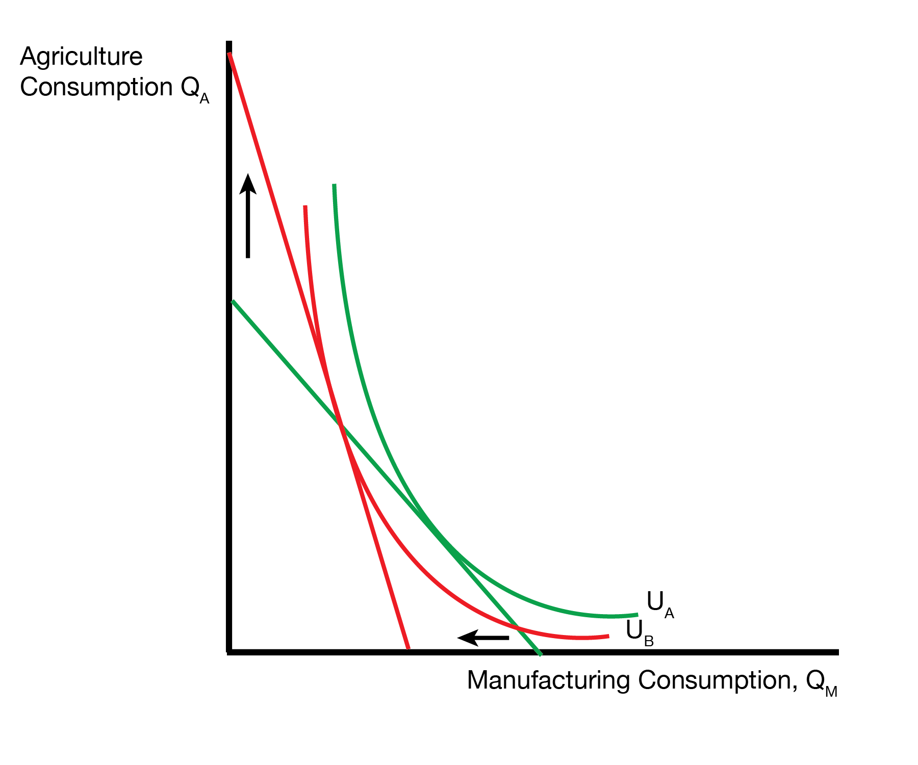
How much manufacturing can a worker afford? They can afford \(W / P_M = (P_M \times MPL_M) / P_M = MPL_M\) units of manufacturing. We know that \(MPL_M\) decreases, so the labor owner can afford less manufacturing. Graphically, this is represented by an inward shift of the manufacturing intercept.
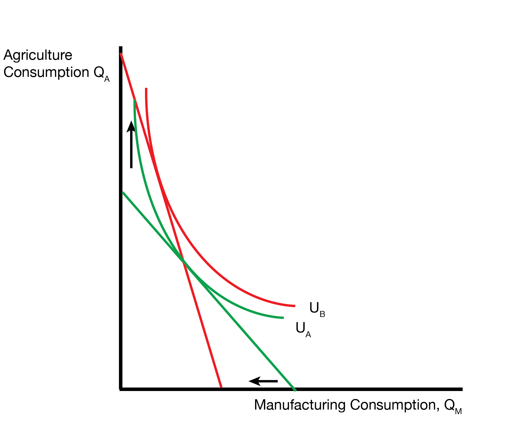
How much agriculture can a worker afford? They can afford \(W / P_A = (P_A \times MPL_A) / P_A = MPL_A\) units of agriculture. We know that \(MPL_A\) increases, so the labor owner can afford more agriculture. Graphically, this is represented by an outward shift of the agriculture intercept.
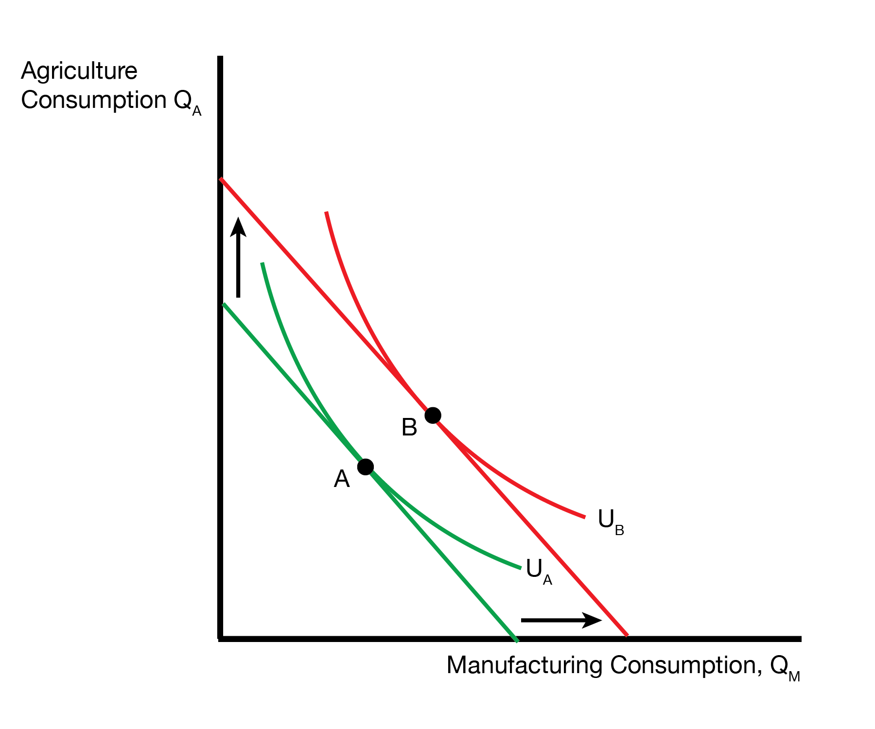
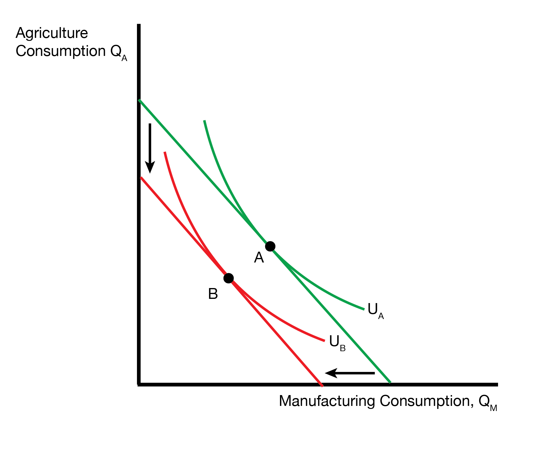
Is labor better or worse off? It depends. The left figure displays the case where labor is better off because it prefers agriculture. The right figure displays the case where labor is worse off because it prefers manufacturing. So the specific factors model not only gives us winners and losers from trade, but it also gives us a range of outcomes for labor.
3.6 Trade Equilibrium
3.7 Conclusion
- We’ve developed a model that features specific factors tied to each industry
- We found the factor specific to the industry with an increasing price (after trade) benefits
- The other factor loses
- The labor case is ambiguous