2 Ricardian Model
Objectives
- Identify comparative advantage and absolute advantage
- Build and identify a Ricardian ‘trade equilibrium’
- Identify gains from trade in the trade equilibrium
- Be able to identify trade flows based on relative prices and comparative advantage
2.1 Introduction
This lecture develops the Ricardian model of trade. We start by developing the autarky (no trade) equilibrium. This involves two steps. First we study preferences which capture what we want to consume. We then study production which says what we can make. This will serve as our baseline. We then develop a free trade equilibrium and examine the following: - Who benefits from trade? - Does everybody benefit from trade? - What drives the pattern of trade flows (who exports and imports which product)?
2.2 Preferences
We will start by making some assumption regarding preferences. Preferences are documented by indifference curves, curves or bundles of curves that give a consumer the same level of utility or satisfaction.
Our preferences are as follows:
- More is better: We prefer to consume more of a good
- Transitivity: If we prefer Z to Y and Y to X, then we prefer Z to X
- Variety: We prefer to consume a variety of goods, so indifference curves are convex
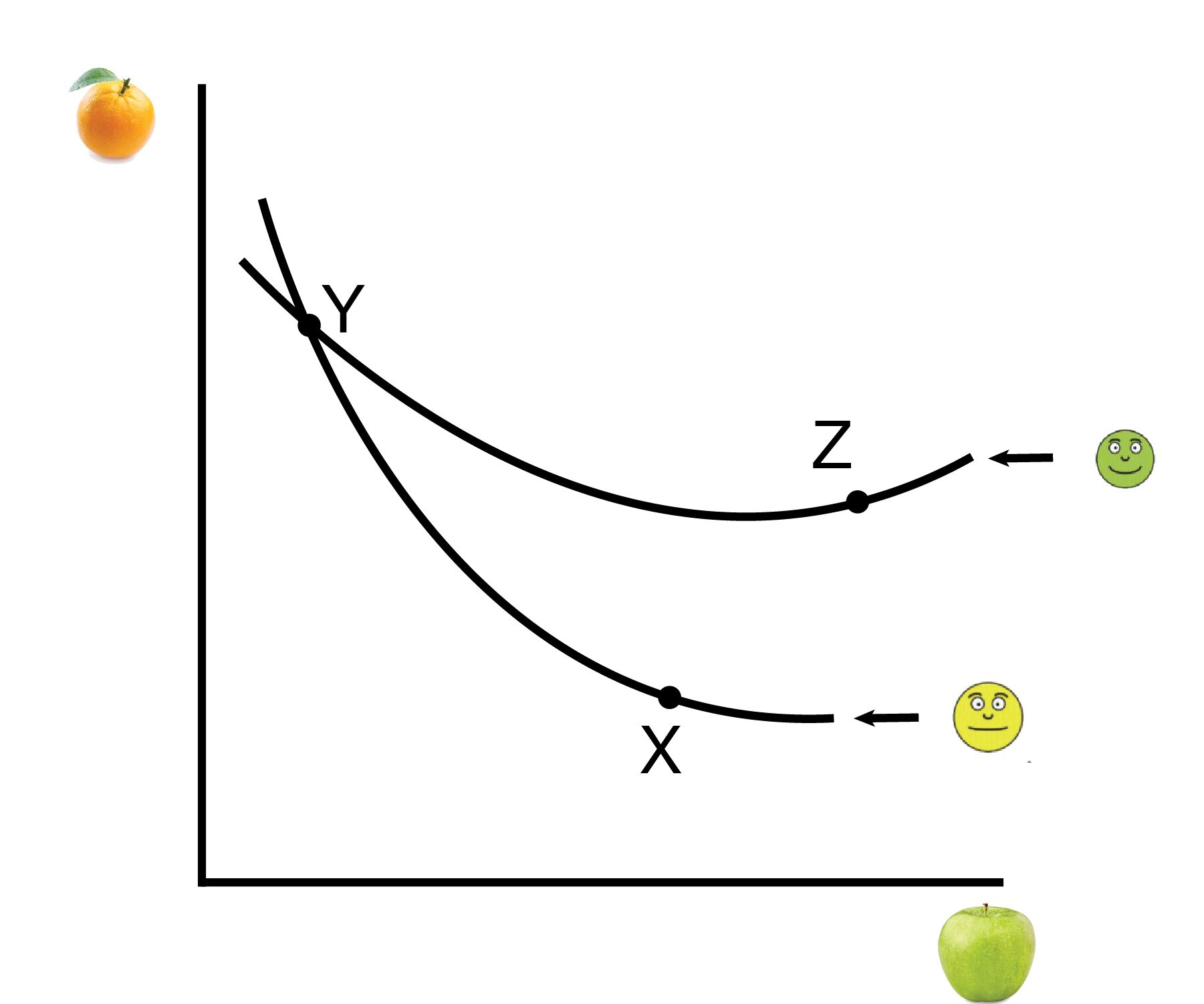
A violation of transitivity is illustrated in the following figure. Note that we are indifferent between Z and Y, are indifferent between Y and X, but prefer Z to X. The transitivity assumption will force that indifference curves (with different levels of satisfaction) do not cross.
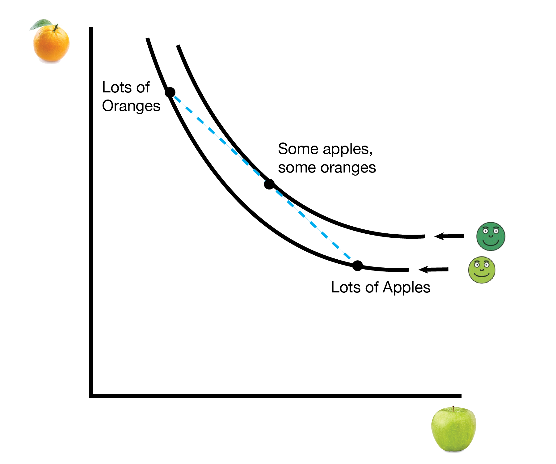
The variety assumption is illustrated in the following figure. Note we have the two extremes: lots of apples or lots of oranges. When we take the ‘average’, or get more variety of apples and oranges, we are better off. This is represented by moving to a higher indifference curve that is associated with more satisfaction. The preference for variety is illustrated by the convex shape of the indifference curves.
When we combine the three assumptions, our indifference curves look like the following:
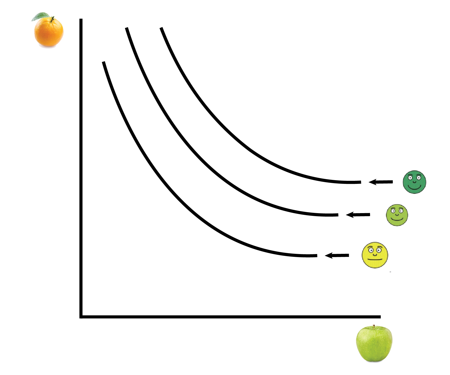
- The indifference curves do not cross
- They are convex
- As we move out from the origin (more apples and oranges), we move to higher indifference curves with higher satisfaction levels.
2.3 Production Possibilities Frontier (PPF)
We’ve laid the foundation for preferences, or how we feel about consuming goods. Now we will turn to production, or how we make goods.
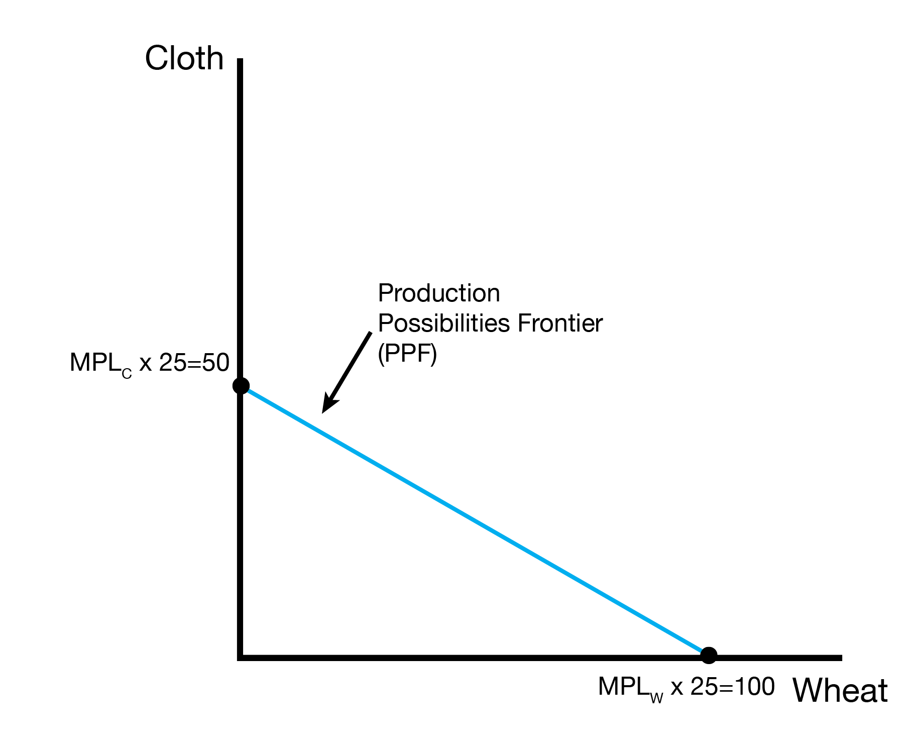
We will assume we have \(L=25\) units of labor that can be used to produce cloth or wheat. The marginal products of labor for each industry are given in the table below.
| Marginal Product of Labor | ||
|---|---|---|
| Home | Foreign | |
| \(MPL_W\) | 4 | 1 |
| \(MPL_C\) | 2 | 1 |
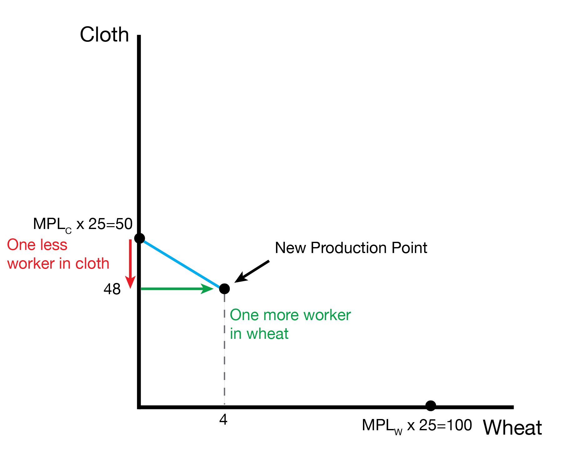
We build the PPF by starting with the extremes: - If we use all our labor to produce cloth, we can produce \(Q_C = MPL_C * L = 2 * 25 = 50\) units of cloth and \(Q_W = 0\) units of wheat. - If we use all our labor to produce wheat, we can produce \(Q_W = MPL_W * L = 4 * 25 = 100\) units of wheat and \(Q_C = 0\) units of cloth. We now move from the extreme of cloth production and consider what happens when we move one worker to the wheat industry. That worker made 2 cloth, so we lose 2 cloth, but that worker can make 4 wheat. As a result, we move from the point (50,0) to the point (48,4). As we iteratively move workers from cloth to wheat, we trace out the full PPF.
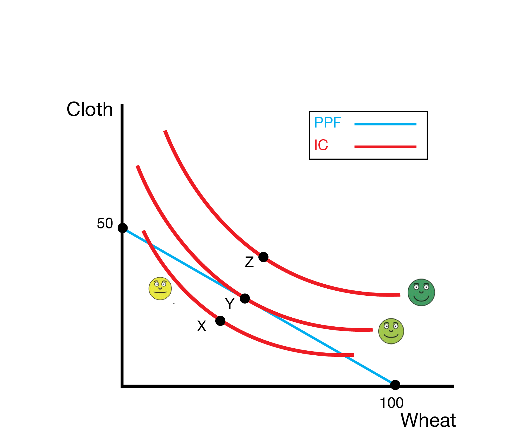
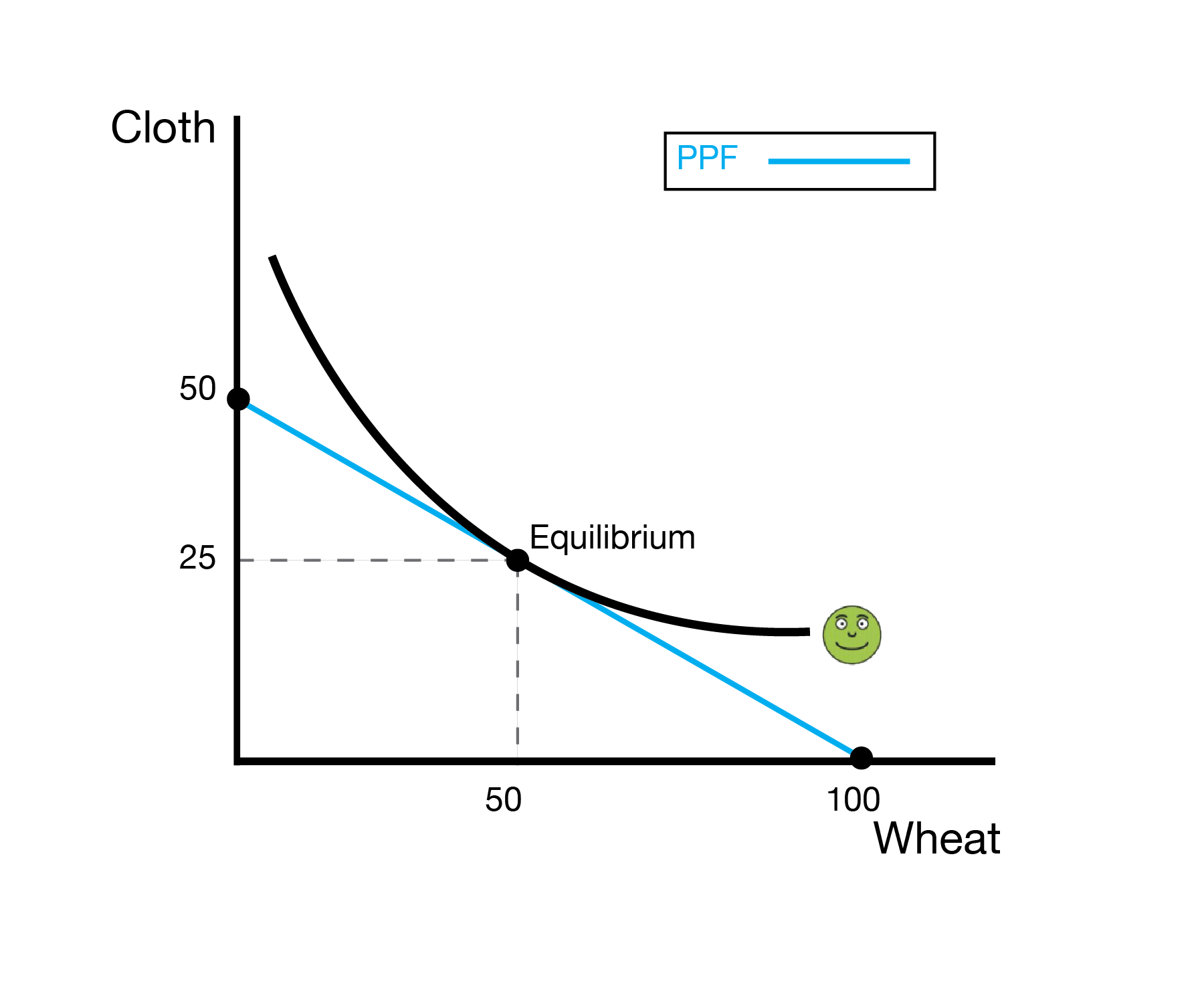
We now combine the PPF (what we can make) with our indifference curves (what we want) to find the autarky equilibrium. In this case, the unique equilibrium is given by point \(Y\). We won’t consume at piont \(A\) because we can reach a higher indifference curve at point \(Y\). We can’t consume at point \(Z\) because it is outside our PPF, so it is infeasible to produce.
2.4 Autarky Equilibrium
We now visit the autarky equilibria for out two countries. We’ve already developed the autarky equilibrium for Home.
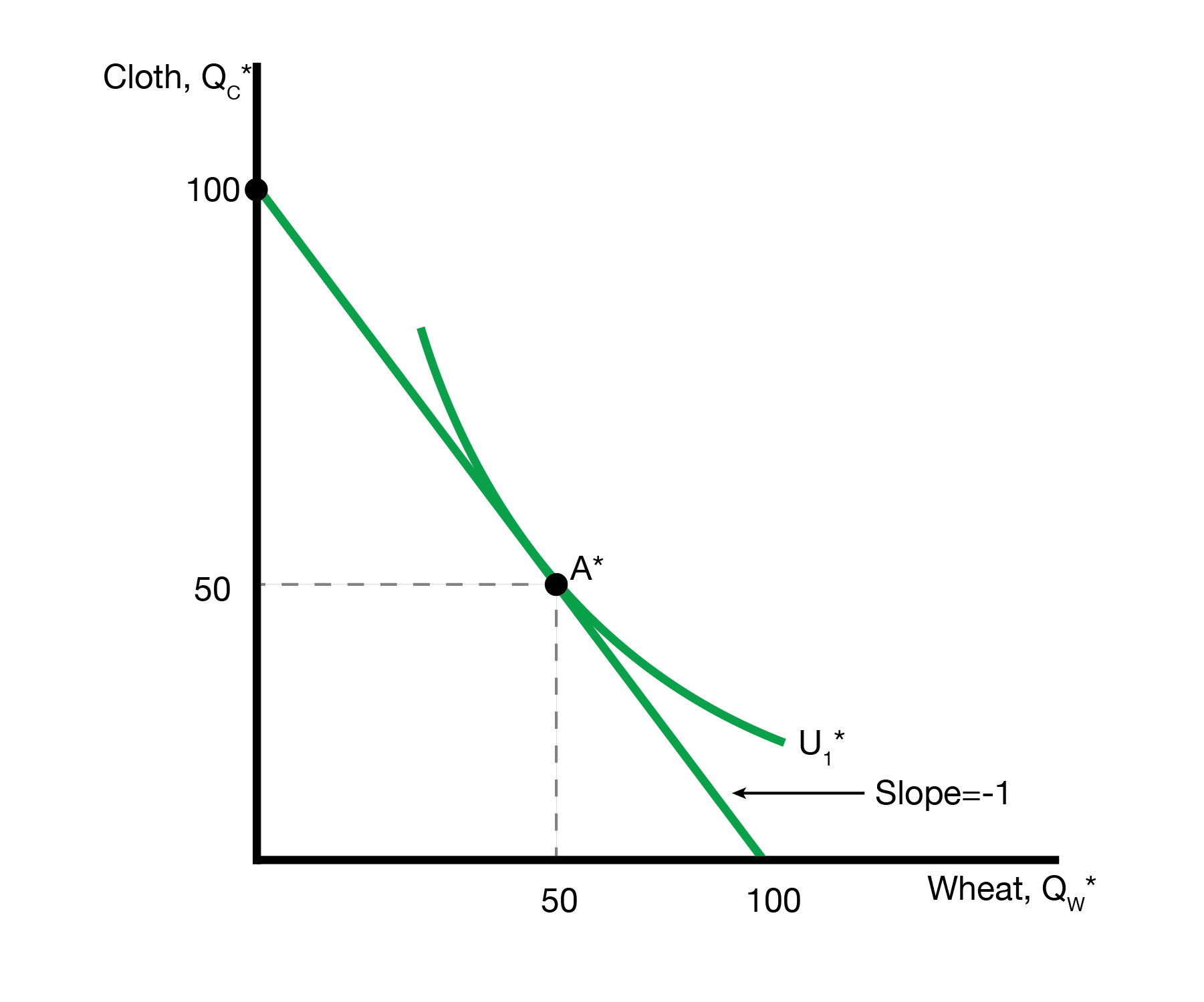
The right figure display’s foreign’s autarky equilibrium (we assume \(L^* = 100\) workers in foreign).
2.5 Trading
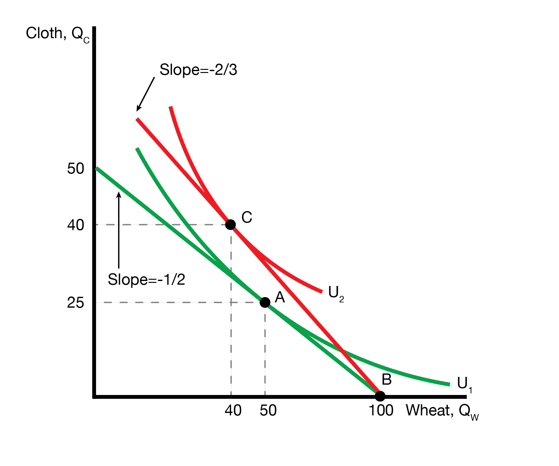
For now we will assume the relative price of wheat is \(P_W / P_C = 2/3\). Home faces two choices: 1) where to produce, and 2) where to consume given their production point. For now we will assume they specialize in their comparative advantage, which is wheat. In this case they produce at point \(B\) on the PPF. Now, households must decide how much to consume. Rather than consuming along the PPF, households trade along the red curve. Critically, the slope is given by the relative price of wheat to cloth, \(P_W / P_C = 2/3\), which is different from the autarky relative price. Given the red curve, households will consume at point \(C\). We know this is the optimal point because it is on the highest indifference curve that is tangent to the red curve.
Our households happier? Yes, we can see point \(C\) is on a higher indifference curve (further from the origin) that the autarky consumption point \(A\).
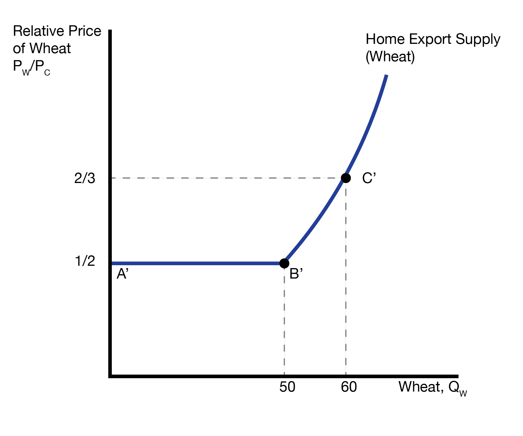
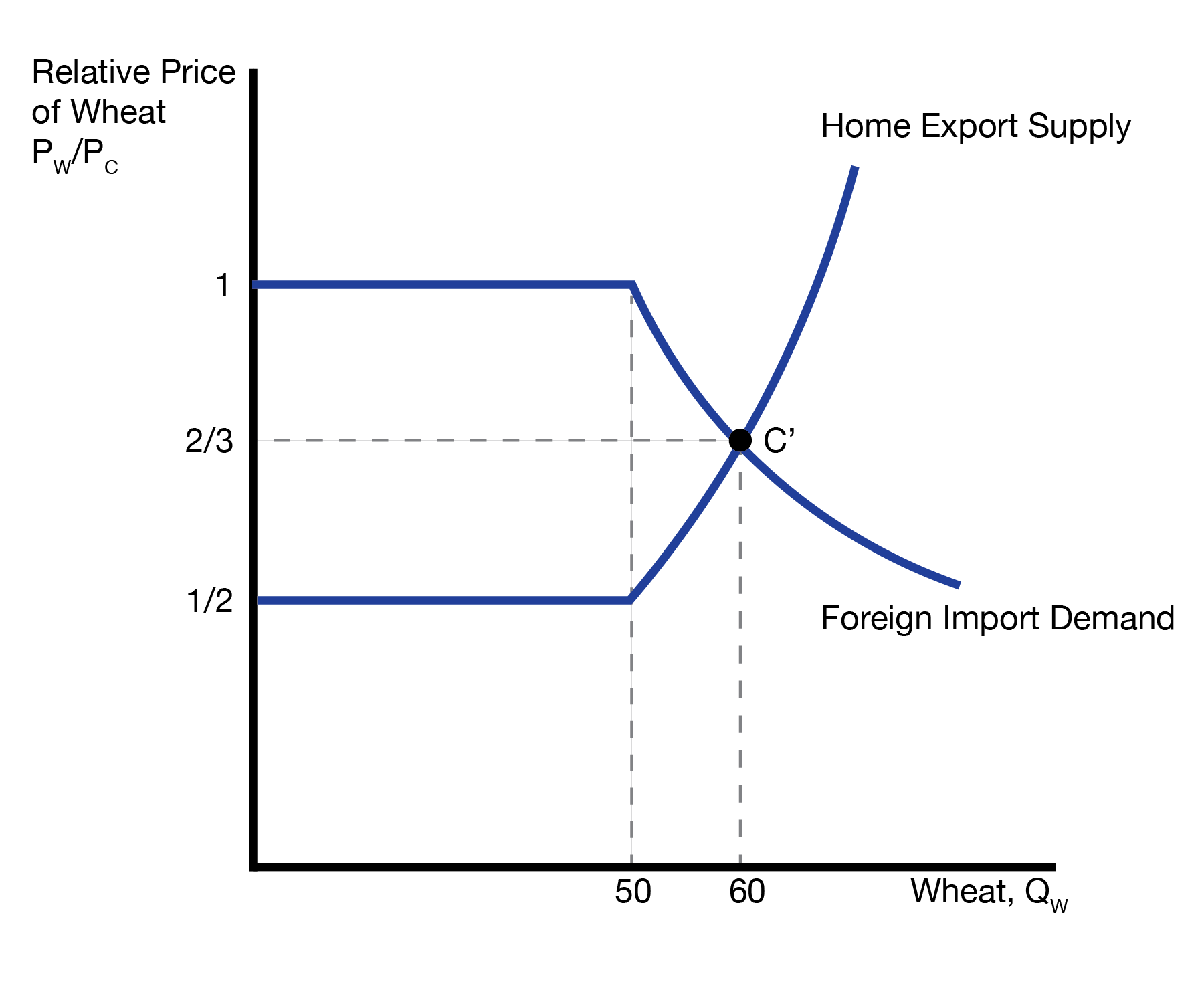
We can show that the steeper the relative price of wheat to cloth, the more wheat home will export. This leads to the home export supply curve.
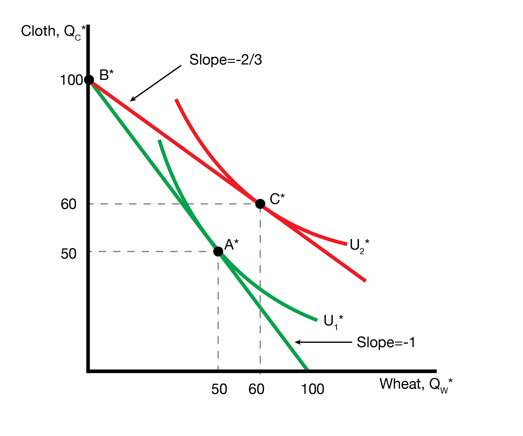
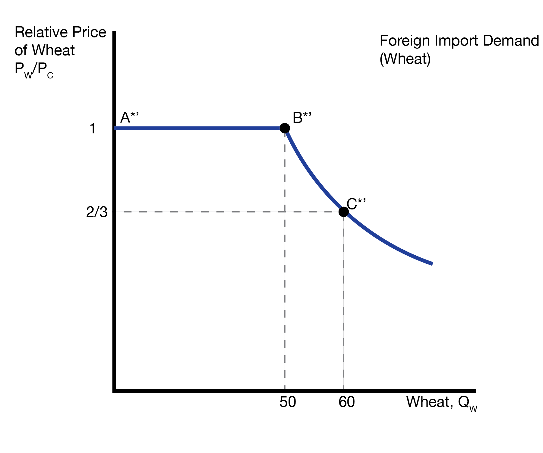
For Foreign, we assume they specialize in their comparative advantage, which is cloth. Foreign produces at point \(B^*\) on their PPF. Households in Foreign then decide how much to consume, trading along the red curve with slope given by the relative price \(P_W / P_C = 2/3\). The optimal consumption point is \(C^*\), where the highest indifference curve is tangent to the red curve. Are Foreign households happier? Yes, point \(C^*\) lies on a higher indifference curve (further from the origin) than the autarky consumption point \(A^*\). As the relative price of wheat to cloth decreases, Foreign imports more wheat. This relationship is captured by the foreign import demand curve.
We bundle the relationship between the relative price and imports and exports into the following definitions:
2.6 Trade Equilibrium
We’re now ready to define the ‘trade’ equilibrium. In this case the price is the relative price of wheat to cloth, \(P_W / P_C\). The ‘good’ is home exports of wheat (foreign imports of wheat). The trade equilibrium is the relative price of wheat and quantity of exports such that the quantity exported by Home equals the quantity imported by Foreign (the market clears). In this case, everbody that wants to sell wheat abroad can, and everybody that wants to buy wheat from abroad can. Note that this is no different from the equilibrium in a competitive market: we find the price that clears the market, given supply and demand.
2.7 Conclusion
- This lecture builds the autarky equilibrium of the Ricardian Model
- We first develop the autarky equilibrium of the Ricardian model in two parts
- First, we develop indifference curves ‘what we want’
- Second, we develop the production possibilities frontier ‘what we can make’
- We then combine the two to form our autarky equilibrium
- We then build the Ricardian trade equilibrium and find that trade flows (imports / exports) depend on relative prices and comparative advantage
- Given the international trade market, both Home and Foreign improved their satisfaction
- Notably, we failed to find any losers of international trade